 Scan for your copy
When the world leaves the training set
A model can be accurate on i.i.d. test data and still fail the moment the input is new, rare, or slightly perturbed. This workbook walks Lecture 13 (out-of-distribution detection), Lecture 14 (contrast data mining), and the Week 8 adversarial demo to the official tutorial answers.
Out-of-distribution detection
Lecture 13, in order. A classifier that is accurate under the i.i.d. assumption can still be wrong and confident once the world moves.
The i.i.d. promise, and when it fails
In the ideal world every training and test pair \((x,y)\) is drawn independently from the same joint distribution. Cross-validation, feature selection, and overfitting arguments all lean on that fact.
\[ P_{\mathrm{test}}(x,y) \;=\; P_{\mathrm{train}}(x,y) \]In the real world the equality fails. The lecture names two shifts. Each plot is the same 2-D feature space: filled points are train, hollow points are test.
i.i.d.
\(P_{\mathrm{test}}(x,y)=P_{\mathrm{train}}(x,y)\). Both splits sit in the same two blobs. This is the promise behind ordinary test accuracy.
Covariate shift
\(P(x)\) changes. The conditional \(P(y\mid x)\) stays fixed. The frog is still a frog, but the pixels are noisier, darker, or more compressed. Used to test generalisation and robustness.
Semantic shift
New classes \(P(y_{\mathrm{new}})\) appear at test time. These are out-of-distribution (OOD) samples. The model should refuse to predict, not assign a training label with high confidence.
Do models know what they don’t know?
This is the lecture figure. Ovadia et al. (NeurIPS 2019) take a clean in-distribution image and corrupt it: noise, blur, compression. The frog is still a frog — same \(P(y\mid x)\) as the covariate-shift scatter above, not a new class. The lecture sentence is two claims, and they are the two panels. Click a thumb, or drag the slider; the highlighted column is the severity you are unpacking.
Unpack the highlighted column. Same 0–1 axis, two different numbers — not two slices of one probability. Green is ① accuracy (top panel). Red is ② ECE (bottom panel): size-weighted \(\lvert\mathrm{acc}-\mathrm{conf}\rvert\), a gap, not leftover confidence you can add to the hit rate.
(top panel)
(bottom panel)
still frog
\(x\): shift intensity
How hard the pixels have been corrupted. Clean (the lecture’s “Test”), then severity 1…5. Not a new label. This is covariate shift.
① Top panel: accuracy drops
Fraction of correct top-1 labels. The boxes fall. That is the first clause of the lecture sentence: more mistakes. You cannot see overconfidence here.
② Bottom panel: ECE rises
ECE is size-weighted \(\lvert\mathrm{acc}-\mathrm{conf}\rvert\) across confidence bins. The boxes rise: the gap grew. ECE is not “extra sure-ness” stacked on accuracy. Overconfidence is the joint reading: accuracy falling while that gap grows. The next section defines the number.
On the figure above, \(x\) is corruption severity. The top panel is accuracy. The bottom panel is ECE — reported there without a definition. The pictures and formulas below follow Maja Pavlovic’s visual introduction Understanding Model Calibration. Figures are reused from that post.
What calibration is
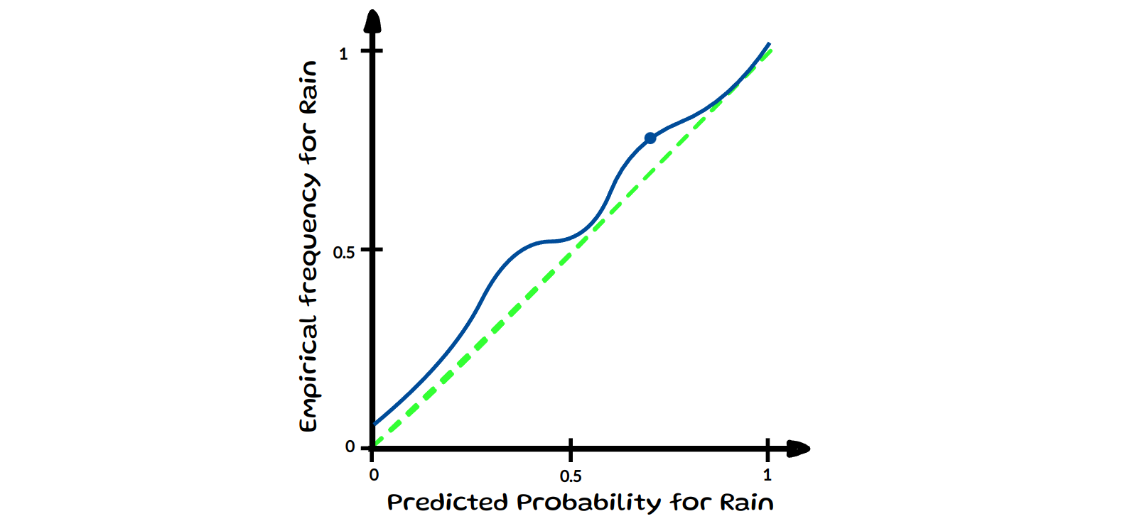
Calibration asks whether a model’s estimated probabilities match real-world frequencies. If a weather model says “70% chance of rain” on many days, then about 70% of those days should actually be rainy (Dawid 1982; DeGroot & Fienberg 1983). The same idea applies to a classifier: a batch of predictions that all report confidence \(c\) should be correct about \(c\) of the time. That is what makes a probability reliable, not just a ranking score.
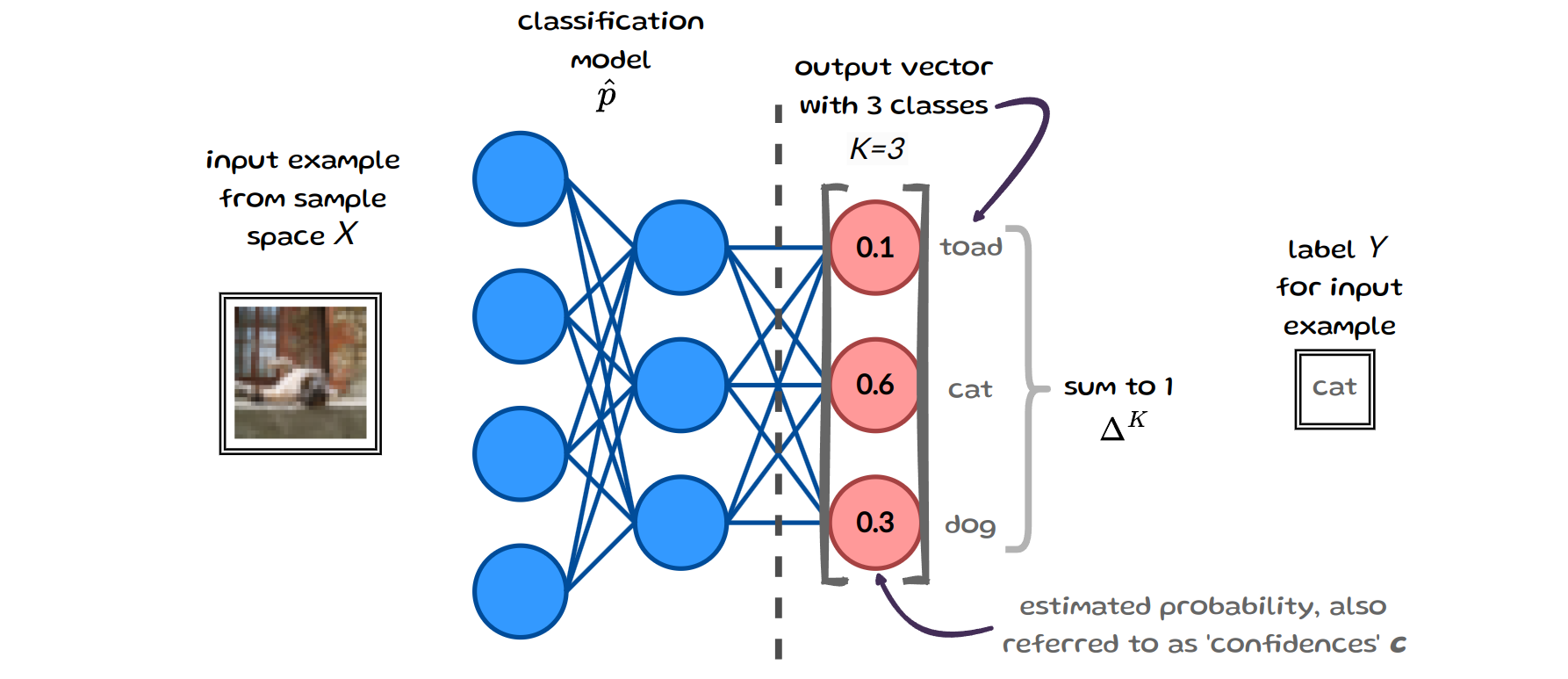
Write \(Y\in\{1,\ldots,K\}\) for the label and \(\hat p:\mathscr{X}\to\Delta^K\) for a classifier that returns a probability vector on the simplex (entries in \([0,1]\), summing to 1). Each coordinate is a confidence that the input belongs to that class.
Confidence calibration
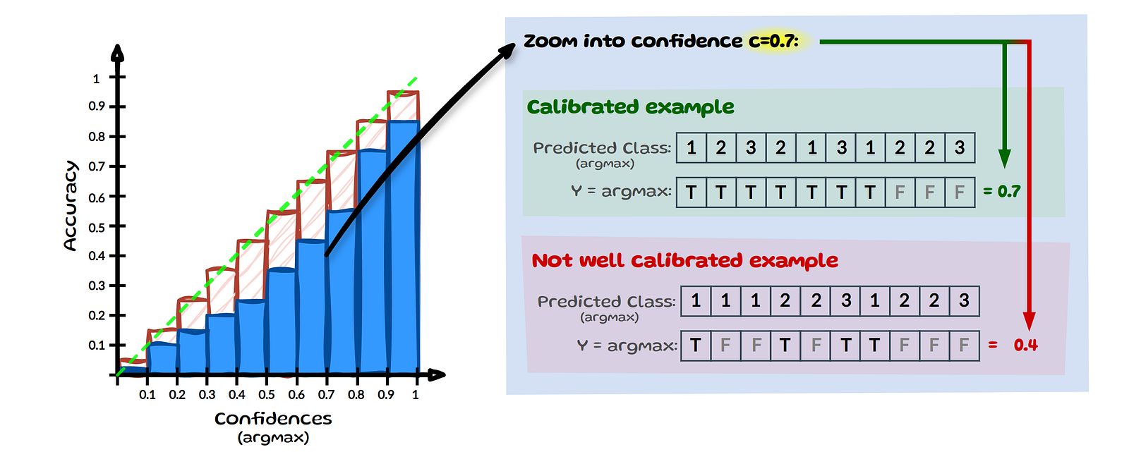
The usual ML definition, formalised by Guo, Pleiss, Sun & Weinberger (ICML 2017) and named confidence calibration by Kull et al. (2019), only looks at the largest entry of \(\hat p(X)\). The model is confidence-calibrated if, at every confidence \(c\), it is correct \(c\) of the time:
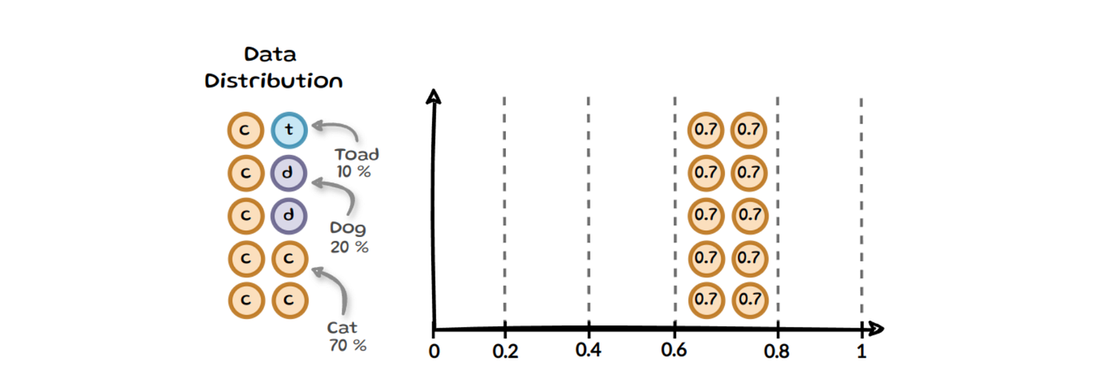
\[ \mathbb{P}\bigl(Y=\arg\max \hat p(X) \;\big|\; \max \hat p(X)=c\bigr) \;=\; c \qquad\forall\, c\in[0,1]. \]Zoom into \(c=0.7\). Take ten inputs whose top probability is 0.7. If seven of those ten predictions are correct, the model is calibrated at 0.7. If only four are correct, it is overconfident at that level. Full calibration requires this for every \(c\), which is the green diagonal of the reliability diagram.
Expected calibration error
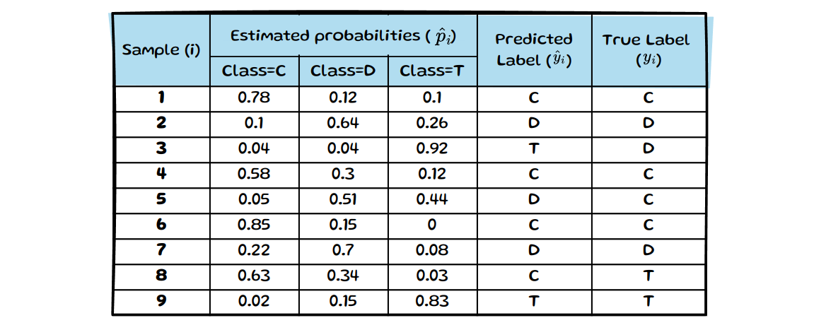
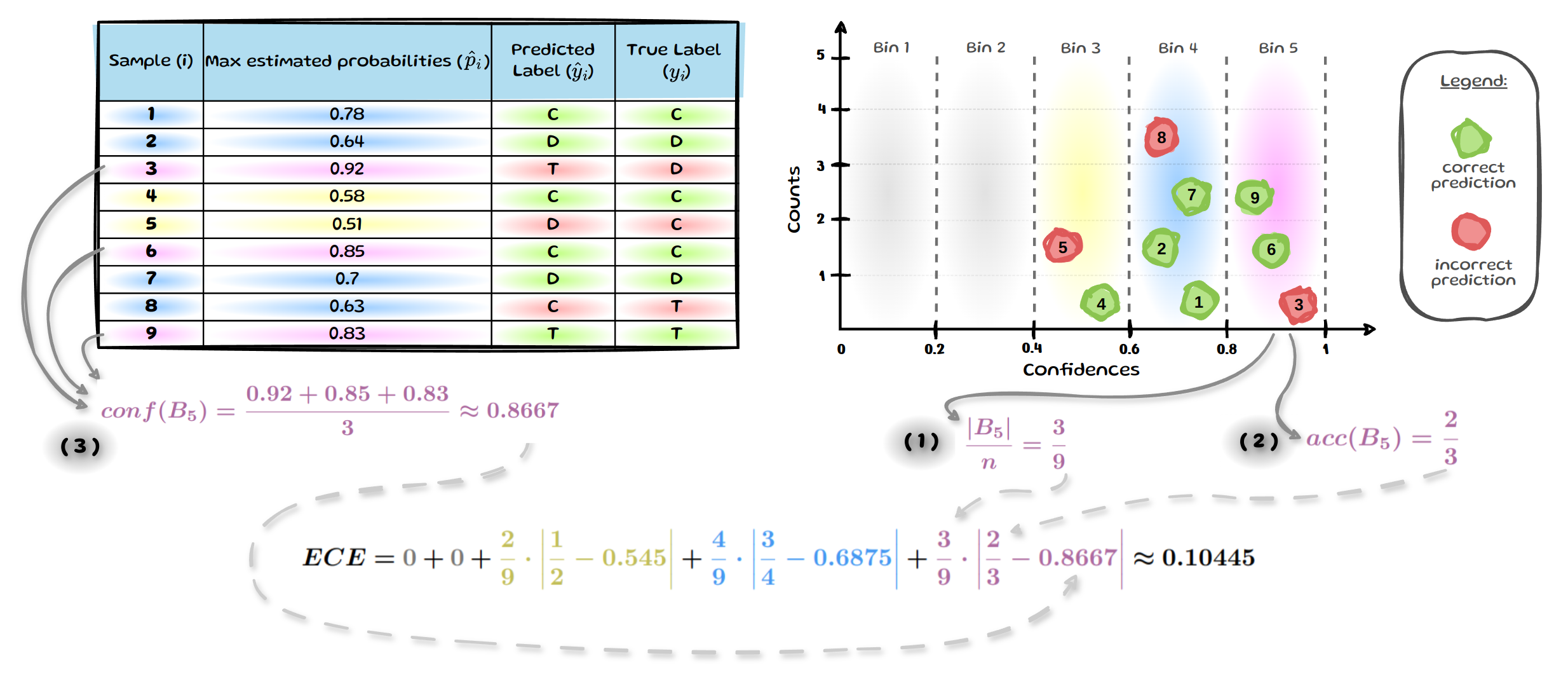
ECE (Naeini, Cooper & Hauskrecht, AAAI 2015; Guo et al., 2017) turns that picture into one number. Split the \(n\) test points into \(M\) equal-width bins \(B_1,\ldots,B_M\) by the maximum probability. In bin \(B_m\), accuracy is the fraction of correct top-1 labels and confidence is the mean of those maxima. ECE is the size-weighted absolute gap:
\[ \mathrm{ECE} \;=\; \sum_{m=1}^{M} \frac{\lvert B_m\rvert}{n} \bigl\lvert \mathrm{acc}(B_m)-\mathrm{conf}(B_m)\bigr\rvert, \] \[ \mathrm{acc}(B_m) \;=\; \frac{1}{\lvert B_m\rvert}\sum_{i\in B_m}\mathbf{1}(\hat y_i=y_i), \qquad \mathrm{conf}(B_m) \;=\; \frac{1}{\lvert B_m\rvert}\sum_{i\in B_m}\max_k \hat p(x_i)_k. \]A perfectly calibrated model has ECE \(=0\). Overconfidence is \(\mathrm{conf}>\mathrm{acc}\) in a bin — the gap that the rising ECE boxes track as shift intensity grows.
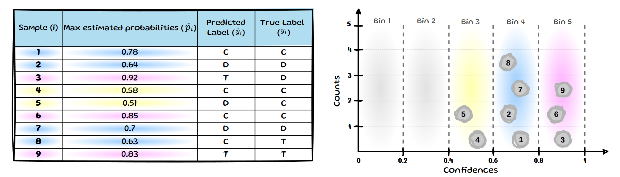
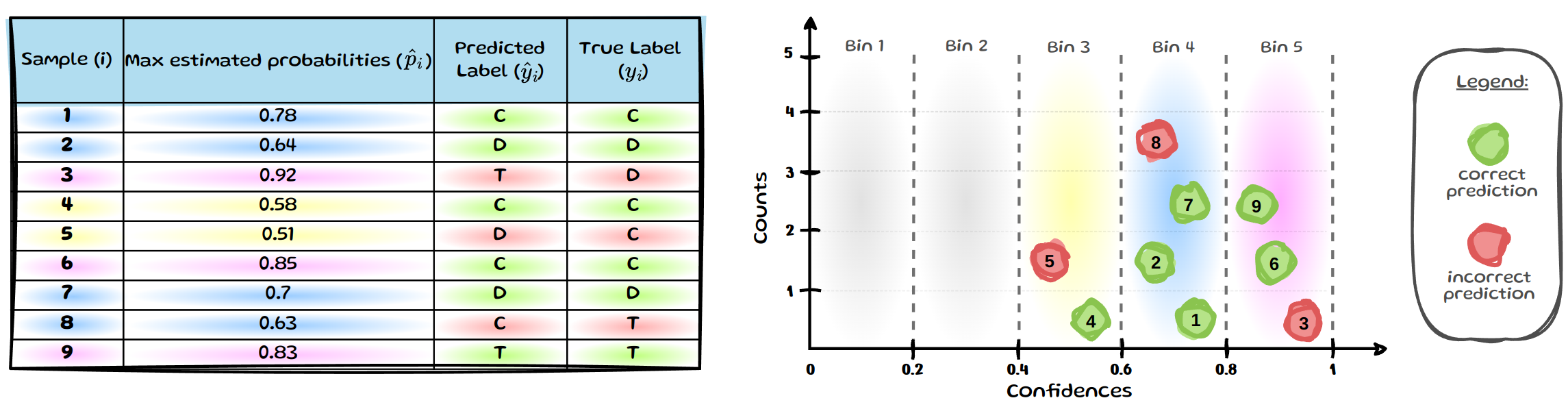
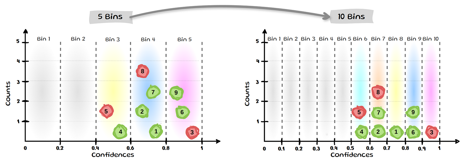
Pavlovic’s nine-sample walk-through makes the bins concrete. Each row is a vector over cat / dog / toad. Only the max probability is binned (\(M=5\) equal-width bins). Green means \(\hat y_i=y_i\); red means a mistake. For bin \(B_5\) one computes the mass \(\lvert B_5\rvert/n\), then \(\mathrm{acc}(B_5)\) and \(\mathrm{conf}(B_5)\). Repeating over all bins in this toy gives \(\mathrm{ECE}=0.10445\).
ECE is still the default number, including on the bottom panel of the Ovadia figure. It is also easy to game. Pavlovic collects the standard objections (Nixon et al.; Kumar et al.; Kull et al.; Vaicenavicius et al.).
Low ECE is not high accuracy
A model that always predicts the majority class at that class’s prevalence has ECE \(=0\) and can still be a bad classifier. Report accuracy (or AUROC, for OOD) alongside ECE.
The bins are a choice
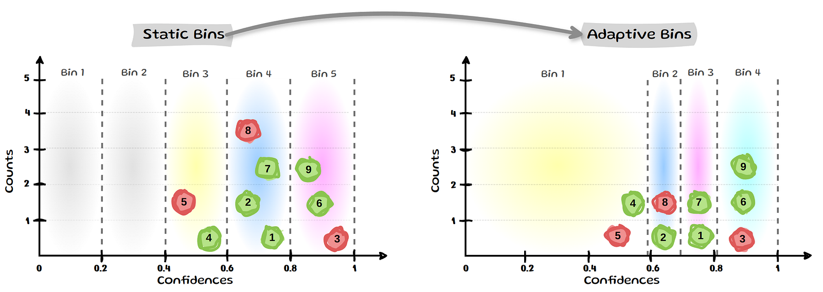
Equal-width bins are sensitive to \(M\). Modern nets dump mass in the last few bins; empty bins contribute 0. Adaptive / equal-mass bins exist (ACE, TACE, ECEsweep).
Only the maximum is used
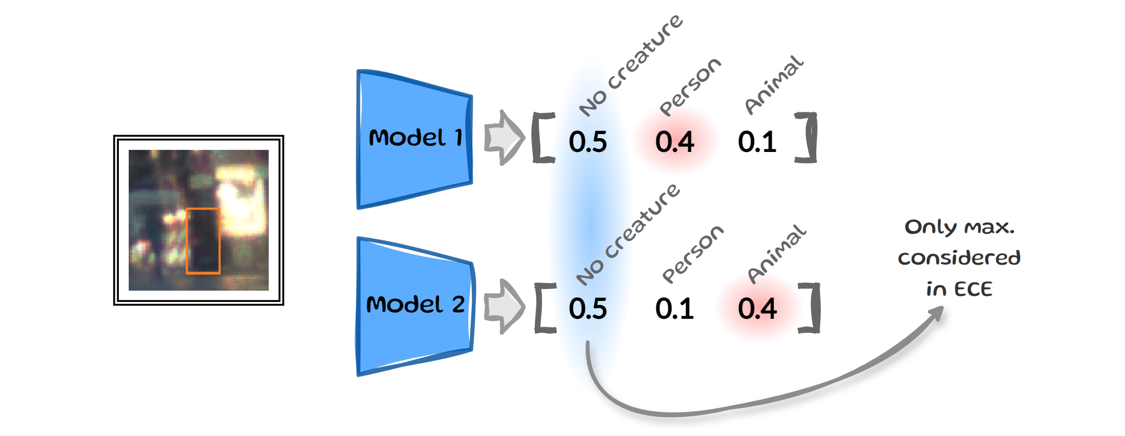
ECE bins \(\max_k \hat p_k\), the same number as MSP. Two softmax vectors with the same peak and different tails look identical to ECE, and would look identical to an MSP OOD detector.
Why accuracy can fall while ECE rises
The Ovadia figure is two summaries of one test set. Accuracy counts how many predictions are right. ECE asks whether the reported probabilities still match that hit rate. The toy below uses the same five equal-width bins as the formula above. Forty confidences are frozen — the net keeps saying the same thing. Only the squares flip from green to red. That is the overconfident-mistake story in one picture.
Each square is one test image, sitting in the bin of its max probability. Green = correct. Red = wrong. The bars underneath are the two numbers ECE compares in that bin: mean confidence (grey) versus accuracy (colour). Drag the same 0…5 severity axis as the frog figure.
Same five bins: accuracy (colour) versus mean confidence (grey), 0–1 scale
(fraction green)
(does not move)
(weighted gaps)
That is why the Ovadia figure stacks accuracy over ECE: under covariate shift the net is both wrong more often and more overconfident (a larger \(\lvert\mathrm{acc}-\mathrm{conf}\rvert\) gap). Real nets can also shift their confidence a little; the lecture’s punchline is the gap, which is what you just watched grow. Later in this primer, MSP is exactly the \(\max_k p_k\) that ECE bins on. For the rest of the blog — multi-class and class-wise calibration, human-uncertainty labels — see Pavlovic (2025).
Accuracy is not confidence
Accuracy is the fraction of predictions that are correct. Confidence is the probability the model assigns to its chosen class. Softmax turns logits \(z_k\) into a distribution over the \(K\) training classes:
\[ p_k \;=\; \frac{e^{z_k}}{\sum_{j=1}^{K} e^{z_j}}, \qquad k=1,\ldots,K. \]The two numbers need not move together. A network can be accurate on i.i.d. data and still output \(p_k \ge 0.996\) on images that are unrecognisable to a human (Nguyen, Yosinski & Clune, CVPR 2015).
Why a DNN is confident far from the data
Distance-aware models should be uncertain in empty regions of input space. A typical deep net is not. Its softmax saturates, so confidence stays high even on points that no training class ever occupied.
The colour is uncertainty, as on the lecture slide: yellow means the model should refuse, purple means it is sure. Left: a distance-aware scorer goes yellow as soon as we leave the moons, so the red blob is refused. Right: a typical net is purple almost everywhere, including on that blob.
A deep generative model trained on a complex dataset can assign higher log-likelihood to a simpler one. Glow trained on CIFAR-10 puts SVHN to the right of the CIFAR-10 histogram: the OOD digits look more typical than the ID photographs.
This is the visual seed of Question 2. Reconstructing well on ID data does not imply reconstructing badly on OOD data, especially when the OOD set is simpler.
The OOD detection objective
Train on an in-distribution (ID) domain, for example CIFAR-10. At test time, score every input so that ID and OOD (for example SVHN) separate. The lecture’s goal:
- Maximise AUROC of the binary ID / OOD decision.
- Keep the false-alarm rate low.
- Have confidence on OOD below confidence on ID.
- No labels on unknowns during training.
- The unknown region of a high-dimensional input space is enormous.
- High-capacity nets make the overconfidence problem worse.
- Density estimation with deep generative models is itself hard (the Glow figure).
- Real images contain many objects, so “in” versus “out” is not always a single label.
Four families of detector
Post-hoc
No extra training. Read a score from a frozen model. Maximum softmax probability; Mahalanobis distance in feature space.
Representation learning
Pre-train (for example a Vision Transformer on ImageNet-21K) and optionally fine-tune so ID and OOD separate in embedding space.
Ensembles
Average independently trained models. Diversity of \(\theta_k\) often improves both accuracy and uncertainty.
Outlier exposure
Train with an auxiliary outlier set so the model is explicitly uncertain on data that is not ID.
Maximum softmax probability (MSP)
Hendrycks & Gimpel (ICLR 2017). The OOD score is the largest softmax entry. An OOD input should, in the ideal case, produce a nearly uniform distribution, so the maximum is close to \(1/K\).
\[ \mathrm{MSP}(x) \;=\; \max_{k=1,\ldots,K} \mathrm{softmax}(z(x))_k. \]CIFAR-10 images go through a network. The detector keeps only \(\max_k p_k\). Flag OOD if that number falls below a threshold \(\tau\).
Mahalanobis distance in feature space
Lee, Lee, Lee & Shin (NeurIPS 2018). Fit a class-conditional Gaussian on the last-layer embedding \(f(x)\) of the training set, with class mean \(\mu_k\) and a shared covariance \(\Sigma\). The score for class \(k\) is the squared Mahalanobis distance
\[ MD_k(x) \;=\; \bigl(f(x)-\mu_k\bigr)^{\mathsf{T}}\Sigma^{-1}\bigl(f(x)-\mu_k\bigr). \]Predict OOD if \(\min_k MD_k(x)\) exceeds a threshold. This uses geometry in representation space, not just the softmax peak.
Click any point. The detector reports \(\min_k MD_k\) and the MSP of a softmax built from the same class means.
Deep ensembles
Lakshminarayanan, Pritzel & Blundell (NeurIPS 2017). Train \(K\) networks with different random seeds and average the categorical distributions:
\[ p(y\mid x) \;=\; \frac{1}{K}\sum_{k=1}^{K} p(y\mid x,\theta_k). \]The mixture is usually better calibrated than any single \(\theta_k\). It is still a training-time method: you pay for \(K\) models at train and at test.
Disagreement among members raises the entropy of the average, which is useful on OOD inputs.
Outlier exposure (OE)
Hendrycks, Mazeika & Dietterich (ICLR 2019). Teach the network to be uncertain on an auxiliary outlier set \(D_{\mathrm{OE}}^{\mathrm{out}}\). For multiclass classification the extra term is cross-entropy toward the uniform distribution \(\mathcal{U}\):
\[ \mathbb{E}_{(x,y)\sim D_{\mathrm{in}}}\bigl[\mathcal{L}(f(x),y)\bigr] \;+\; \lambda\,\mathbb{E}_{x'\sim D_{\mathrm{OE}}^{\mathrm{out}}}\bigl[\mathcal{L}(f(x'),\mathcal{U})\bigr]. \]The first term is ordinary classification loss. The second is the OE loss. Real, diverse outliers (Tiny ImageNet scale, often a 1:2 inlier-to-outlier ratio) help the rule generalise to new OOD sets. The method is sensitive to the choice of \(D_{\mathrm{OE}}\).
Fort, Ren & Lakshminarayanan (NeurIPS 2021) fine-tune a Vision Transformer pretrained on ImageNet-21K. Fewer than 100 outlier images per class already move OOD detection a long way, because the embedding is already linearly separable.
Self-supervised rotation as an OOD score
Hendrycks et al. (NeurIPS 2019). A second head never sees class labels. It only answers: which of four rotations was applied? Toggle ID vs OOD in the pipeline. The normality score is the sum of probability on the true rotation — large \(s(x)\) means ID. (The lecture slide calls this an anomaly score; the formula’s polarity is the opposite.)
\[ s(x) \;=\; \sum_{r\in\{0^\circ,90^\circ,180^\circ,270^\circ\}} p_{\mathrm{rot}}\bigl(r \mid \mathrm{rotate}(x,r)\bigr). \]Same image, four copies. Each copy is rotated, passed through a shared ConvNet \(F(\cdot)\), and scored as a 4-way rotation classification. The green bar is the true rotation — the term that enters \(s(x)\). Toggle ID vs OOD.
(max 4)
A richer variant also sums over vertical translations \(\mathcal{T}_v\) and horizontal translations \(\mathcal{T}_h\). Write \(G_{s,t}(x)\) for the image after those two shifts, then score the applied rotation and translations:
\[ \sum_{r\in\mathcal{R}}\sum_{s\in\mathcal{T}_v}\sum_{t\in\mathcal{T}_h} \Bigl( p_{\mathrm{rot}}\bigl(r \mid \mathrm{rotate}(G_{s,t}(x),r)\bigr) + p_{\mathrm{vert}}\bigl(s \mid G_{s,t}(x)\bigr) + p_{\mathrm{horiz}}\bigl(t \mid G_{s,t}(x)\bigr) \Bigr). \]Shift first (\(G_{s,t}\)), then rotate. Three heads see the applied transform: rotation, vertical shift, horizontal shift. The inner sum adds those three probabilities for every \((r,s,t)\).
A close-up of zebra stripes classifies as “zebra” either way up. Deciding whether the animal is flipped requires modelling the whole shape. Auxiliary rotation therefore pushes the network toward features that are more robust under shift.
Virtual outlier synthesis (VOS)
Du, Wang, Cai & Li (ICLR 2022). Do not fetch an external outlier set. Model the backbone features of each ID class as a Gaussian and sample virtual outliers from the low-likelihood region. That is cheaper than sampling in pixel space.
Given training objects \((x_i, b_i, y_i)\) with hidden vector \(h(x_i,b_i)\) (the box \(b_i\) is used in detection), the class mean and shared covariance are
\[ \hat\mu_k \;=\; \frac{1}{N_k}\sum_{i:y_i=k} h(x_i,b_i), \qquad \hat\Sigma \;=\; \frac{1}{N}\sum_k\sum_{i:y_i=k} \bigl(h(x_i,b_i)-\hat\mu_k\bigr)\bigl(h(x_i,b_i)-\hat\mu_k\bigr)^{\mathsf{T}}. \]Virtual outliers \(\nu_k\) for class \(k\) are draws whose Gaussian density falls below a small \(\epsilon\):
\[ \mathcal{V}_k \;=\; \Bigl\{ \nu_k \;\Big|\; \tfrac{1}{(2\pi)^{m/2}|\hat\Sigma|^{1/2}} \exp\bigl(-\tfrac12 (\nu_k-\hat\mu_k)^{\mathsf{T}}\hat\Sigma^{-1}(\nu_k-\hat\mu_k)\bigr) \;<\; \epsilon \Bigr\}. \]The training objective adds an uncertainty loss to classification and localisation:
\[ \min_\theta\; \mathbb{E}_{(x,b,y)\sim\mathcal{D}} \bigl[\mathcal{L}_{\mathrm{cls}}+\mathcal{L}_{\mathrm{loc}}+\beta\cdot\mathcal{L}_{\mathrm{uncertainty}}\bigr], \] \[ \mathcal{L}_{\mathrm{uncertainty}} \;=\; \mathbb{E}_{\nu\sim\mathcal{V}}\Bigl[-\log\frac{1}{1+e^{-\phi(E(\nu;\theta))}}\Bigr] \;+\; \mathbb{E}_{x\sim\mathcal{D}}\Bigl[-\log\frac{e^{-\phi(E(x;\theta))}}{1+e^{-\phi(E(x;\theta))}}\Bigr]. \]The first term pushes virtual outliers toward the “uncertain” side of a logistic. The second term pushes real ID objects toward the “certain” side.
Filled dots are ID features. Open rings are virtual outliers drawn where the Gaussian density is below \(\epsilon\). Those rings regularise the decision boundary so a moose on the road is not called “car, 99%”.
Udayangani, Dolatabadi, Erfani & Leckie (WACV 2025). When ID classes are imbalanced, a pretrained backbone is Gaussianised, a \(k\)-NN graph is built, and a GCN refines embeddings before a linear classifier. Rare ID classes are no longer confused with OOD as easily.
Anomaly detection versus OOD detection
What are differences between anomaly detection and OOD detection?
Both tasks flag inputs that are not “normal”. They do not ask the same question. Anomaly detection looks for rare or irregular points inside one dataset. OOD detection asks whether a point could have been drawn from the training distribution of a deployed model, and is especially about overconfident neural nets on new classes or new domains.
Each card is one scene. Choose anomaly or OOD. The official distinction is the goal, not the algorithm.
Why autoencoders are not OOD detectors
One of the most powerful methods for anomaly detection is AE and VAE, but why we cannot use them directly for OOD detection?
An autoencoder is trained to reconstruct ID points. Reconstruction error is a good anomaly score when anomalies are harder to reconstruct than normals. That need not hold for OOD data. Nalisnick et al. showed that a density model trained on CIFAR-10 can assign higher likelihood to SVHN. The same geometry appears in reconstruction: a decoder trained on complex photographs can copy a simple digit almost perfectly.
The network was trained on a textured ID patch (CIFAR-like). Slide between that patch and a simpler OOD digit (SVHN-like). Reconstruction error can fall, not rise.
error (MSE)
error at 0.12
Off-the-shelf versus custom detectors
What are the different off-the-shelf custom OOD detection techniques discussed in the class and their differences?
Off-the-shelf (post-hoc) methods read a score from a model that is already trained. Custom methods change training: extra losses, extra data, or extra models. Sort the lecture’s methods into the two bins.
Off-the-shelf · post-hoc
Custom · training-time
MSP and Mahalanobis need no extra training. OE, ensembles, and VOS do.
A CIFAR-10 versus SVHN lab
Implement an Out-Of-Distribution (OOD) detection technique and train it using the CIFAR-10 dataset for in-distribution data, and use appropriate measures to evaluate its performance on OOD detection from the SVHN datasets.
ID domain: CIFAR-10. OOD domain: SVHN. Score every test point, draw ID and OOD histograms, and report AUROC (higher is better) together with a false-alarm rate at a fixed recall. This page runs the same protocol on a 2-D stand-in so the numbers move in class. The LMS PyTorch notebook is the place to train a real CIFAR-10 network.
(TPR)
(FPR on ID)
AUROC is threshold-free: it is the probability that a random OOD point scores more “OOD-like” than a random ID point. TPR and FPR depend on \(\tau\).
Contrast data mining
Lecture 14. This material is not on the tutorial sheet. It is the second lecture of the week, and it ends with “Next: Adversarial Machine Learning”.
To contrast is “to compare or appraise in respect to differences”. Contrast data mining finds patterns and models that distinguish two or more datasets or conditions. The representation should be interpretable, non-redundant, and tractable; the quality should be statistically significant and rankable.
Time
Yesterday’s traffic versus today’s.
Space
Human DNA at locus \(x\) versus mouse DNA at locus \(x\).
Rank
High-income versus low-income earners.
Class
Brown hair versus blonde hair; or a statement that holds only inside one profession.
Typical uses: report a significant change, raise an alert when a dissimilarity index falls below a threshold, build one-class or multi-class classifiers, and synthesise extra instances of a rare class.
Network flows, summarised then contrasted
Anomaly detectors rank thousands of flows. Analysts read the first pages. A compact report is a trade-off between compaction gain and information loss. Clustering can replace five TCP/80 rows by one summary with wildcards. Contrast mining then asks what changed between Day 1 and Day 2: new UDP/90 destinations, a new source, a jump in bytes.
Support, and the Apriori principle
An itemset is a set of items; a \(k\)-itemset has size \(k\). \(\mathrm{Count}(X,D)\) is the number of transactions in \(D\) that contain \(X\). Support is the corresponding fraction:
\[ \mathrm{support}(X,D) \;=\; \frac{\mathrm{Count}(X,D)}{|D|}. \]\(X\) is frequent when its support count \(\mathrm{Count}(X,D)\) is at least a threshold \(\mathrm{minsup}\), equivalently \(\mathrm{support}(X,D)\ge\mathrm{minsup}/|D|\). Han’s example below uses \(\mathrm{minsup}=2\) as a count (so \(\mathrm{support}\ge 2/9\)). Apriori grows frequent itemsets by length. The pruning rule is the Apriori principle:
If an itemset is infrequent, then every superset of it is infrequent. Once \(AB\) fails the threshold, \(ABC\), \(ABD\), \(ABE\), and every longer set that contains \(AB\) can be discarded without counting.
Edges are covering relations (add one item). \(AB\) itself is counted and fails. Grey nodes are supersets of \(AB\): dashed edges into them are never followed. That is why Apriori is faster than enumerating every subset — and why it still struggles when there are \(10^4\) frequent 1-itemsets, which spawn more than \(10^7\) candidate 2-itemsets.
FP-growth: one tree, two scans
Han, Pei & Yin. Compress the database into a frequent-pattern tree and grow patterns from it. No candidate generation. Two database scans. Each node stores an item name, a count, and a node-link to the next node of the same item. The header table stores, for each frequent item, its total count and the head of that node-link list.
The lecture’s running example (support-count threshold \(\mathrm{minsup}=2\), i.e. \(\mathrm{support}\ge 2/9\)) is the standard nine-transaction database:
| TID | Items | Ordered frequent items |
|---|
Scan 1 counts items: \(I_2{:}7\), \(I_1{:}6\), \(I_3{:}6\), \(I_4{:}2\), \(I_5{:}2\). All five meet the count threshold 2, so none are dropped. Scan 2 inserts each transaction reordered by that list.
Start at the bottom of the header table. For each item, collect its prefix paths as a conditional pattern base, build a conditional FP-tree on items that are still frequent in that base, and recurse. Concatenate the suffix with every pattern from the conditional tree.
| Item | Conditional pattern base | Conditional FP-tree | Frequent patterns |
|---|---|---|---|
| \(I_5\) | \(\{I_2 I_1{:}1,\; I_2 I_1 I_3{:}1\}\) | \(\langle I_2{:}2,\; I_1{:}2\rangle\) | \(\{I_2 I_5{:}2\},\;\{I_1 I_5{:}2\},\;\{I_2 I_1 I_5{:}2\}\) |
| \(I_4\) | \(\{I_2 I_1{:}1,\; I_2{:}1\}\) | \(\langle I_2{:}2\rangle\) | \(\{I_2 I_4{:}2\}\) |
| \(I_3\) | \(\{I_2 I_1{:}2,\; I_2{:}2,\; I_1{:}2\}\) | \(\langle I_2{:}4,\; I_1{:}2\rangle,\;\langle I_1{:}2\rangle\) | \(\{I_2 I_3{:}4\},\;\{I_1 I_3{:}4\},\;\{I_2 I_1 I_3{:}2\}\) |
| \(I_1\) | \(\{I_2{:}4\}\) | \(\langle I_2{:}4\rangle\) | \(\{I_2 I_1{:}4\}\) |
Bottleneck of the tree: sharing the header links makes a parallel implementation wait on shared memory. The gain is still large: two file reads to build the tree, versus one scan per Apriori iteration and a candidate explosion at length 2.
Emerging and jumping patterns
Given a positive (target) dataset \(D_p\) and a negative (source) dataset \(D_n\), the growth rate of pattern \(X\) is
\[ \mathrm{gr}(X,D_p) \;=\; \begin{cases} 0 & \text{if }\mathrm{support}(X,D_p)=\mathrm{support}(X,D_n)=0,\\[4pt] \infty & \text{if }\mathrm{support}(X,D_n)=0\text{ and }\mathrm{support}(X,D_p)>0,\\[4pt] \dfrac{\mathrm{support}(X,D_p)}{\mathrm{support}(X,D_n)} & \text{otherwise.} \end{cases} \]If \(\mathrm{gr}(X,D_p)\ge\rho\) with \(\rho>1\), then \(X\) is an emerging pattern (also called a contrast pattern or a discriminative pattern) for \(D_p\). The infinite case is a jumping emerging pattern (JEP). When \(|D_p|=|D_n|\) the support ratio equals the count ratio, which is why the eight-row example below can be read from counts.
Positive \(D_p\)
| src | dst | pro | pkts | |
|---|---|---|---|---|
| T1 | .22.1 | .10.1 | udp | [2,20] |
| T2 | .55.2 | .10.4 | udp | [40,68] |
| T3 | .22.1 | .10.1 | tcp | [2,20] |
| T4 | .20.1 | .10.2 | tcp | [2,20] |
Negative \(D_n\)
| src | dst | pro | pkts | |
|---|---|---|---|---|
| T1 | .44.2 | .10.2 | tcp | [40,68] |
| T2 | .20.1 | .10.2 | tcp | [2,20] |
| T3 | .20.1 | .10.2 | tcp | [2,20] |
| T4 | .22.1 | .10.1 | udp | [2,20] |
C1 \(\{\mathrm{src}{=}.22.1,\;\mathrm{dst}{=}.10.1,\;\mathrm{pkts}{=}[2,20]\}\) occurs twice in \(D_p\) (T1, T3) and once in \(D_n\) (T4), so \(\mathrm{gr}=2/1=2\). It is an emerging pattern. C2 \(\{\mathrm{src}{=}.55.2,\;\mathrm{dst}{=}.10.4,\;\mathrm{udp},\;\mathrm{pkts}{=}[40,68]\}\) occurs once in \(D_p\) and never in \(D_n\), so \(\mathrm{gr}=\infty\). It is a JEP. (The slide typesets C2’s packet bin as \([2,20]\); the matching positive row is T2, whose bin is \([40,68]\).)
Attack ratio, OCLEP, and a different kind of report
In network traffic, let \(D_{\mathrm{pos}}(\mathrm{att})\) be the attack-labelled subset of the positive data. The attack ratio of a contrast pattern \(X\) is
\[ \mathrm{AttackRatio}(X) \;=\; \frac{\mathrm{Count}(X,D_{\mathrm{pos}}(\mathrm{att}))}{\mathrm{Count}(X,D_{\mathrm{pos}})}. \]High growth rate is strongly associated with attack patterns. In the traffic study most contrast patterns are pure (they sit entirely in attack or entirely in normal); the share of attack patterns rises with the growth-rate threshold.
OCLEP scores a point by the length of its shortest emerging pattern against the training class. A test point from the same class tends to produce long (often empty-of-short) EPs; a point from a different class tends to produce short ones. The lecture’s ROC sits next to one-class SVM.
Anomaly detection model
Learn “normal” from history. Score the current data. Emit anomalies. The output is a list of points.
Contrast mining model
Compare current data to history. Extract significant changes. Emit a short report of patterns, not a long ranked list.
Adversarial examples
Lecture 14 closes with “Next: Adversarial Machine Learning”. Questions 5–7 and the LMS notebook live here. A full attack lecture is later; this primer is the minimum that makes the hog demo and the official Q6 reasons make sense.
An adversarial example is an input \(x'\) that a human still reads as the original class, while a trained model \(f\) changes its prediction. Two boxes, not one. The perturbation has an \(\ell_\infty\) budget \(\varepsilon\) (largest change in any pixel channel). For images the result must also stay a legal pixel, otherwise the attack is using out-of-gamut values that a camera or PNG loader would clip away:
\[ x' \;=\; \mathrm{clip}(x+\delta,\,0,\,1), \qquad \lVert \delta \rVert_\infty \le \varepsilon, \qquad \lVert \delta \rVert_\infty \;=\; \max_i \lvert \delta_i \rvert. \]A white-box attacker has the model, its weights, and its gradients. A black-box attacker has only queries. The LMS notebook is white-box: it back-propagates through ResNet-50.
As discussed in class: (1) distribution differences — the attacker leaves the training measure while staying close in pixel space; (2) insufficient data — the training set does not cover the \(\varepsilon\)-ball around each point; (3) unnecessary features — the net uses brittle directions that a human does not use. Goodfellow, Shlens & Szegedy argue that (3) is largely linearity: in high dimension, many tiny aligned steps add up.
Untargeted, targeted, and FGSM
Let \(\mathcal{L}\) be the training loss (cross-entropy) and \(y\) the true label. An untargeted attack maximises that loss inside the box:
\[ \max_{\lVert\delta\rVert_\infty\le\varepsilon}\; \mathcal{L}\bigl(f(x+\delta),\, y\bigr). \]A targeted attack pushes the prediction toward a chosen class \(y_t\). The notebook does this by maximising loss on the true class and minimising loss on the target at the same time. PyTorch SGD minimises that combined loss:
\[ \min_{\lVert\delta\rVert_\infty\le\varepsilon} \Bigl( -\mathcal{L}\bigl(f(x+\delta),\, y\bigr) + \mathcal{L}\bigl(f(x+\delta),\, y_t\bigr) \Bigr). \]For softmax cross-entropy that difference is just a logit gap. The log-sum-exp normaliser cancels:
\[ \log p_y - \log p_{y_t} \;=\; z_y - z_{y_t}. \]Every other class \(k\notin\{y,y_t\}\) can float. The notebook still uses this objective because it is cheap and matches the LMS cell; a stricter targeted attack would also suppress those other logits (for example Carlini–Wagner).
The fast gradient sign method (Goodfellow et al., 2015) is a one-step linearisation of the untargeted problem. Take the sign of the loss gradient with respect to the input, and step \(\varepsilon\):
\[ x' \;=\; x \;+\; \varepsilon\,\mathrm{sign}\bigl(\nabla_x J(\theta,x,y)\bigr). \]Iterating the sign step with a smaller size, projecting \(\delta\) back onto the \(\ell_\infty\) box, and clipping \(x'\) to \([0,1]\), is projected gradient descent (PGD / BIM). The LMS notebook is milder: ordinary SGD on the raw \(\nabla_\delta\) of that loss, then delta.clamp_(-ε, ε). Sign-normalised PGD keeps taking full-size steps after softmax saturates; unnormalised SGD shrinks. The 2-D widget in Q7 copies the notebook’s SGD, not PGD.
Take a hog logit \(z=w^\top x\). Untargeted FGSM follows \(\mathrm{sign}(\nabla_x\mathcal{L})\), which lowers \(z\): \(\delta=-\varepsilon\,\mathrm{sign}(w)\). Every coordinate then subtracts, \(\Delta z=-\varepsilon\lVert w\rVert_1\approx-\varepsilon\,\lvert w\rvert\,d\). Random \(\pm\varepsilon\) mostly cancel, \(\lvert\Delta z\rvert\sim\varepsilon\,\lvert w\rvert\sqrt{d}\). Drag \(d\) up to ImageNet (\(d=224\times 224\times 3=150{,}528\)). Picture space stays quiet; the hog logit falls.
\(+\varepsilon\)\(-\varepsilon\)not in the sum
What adversarial attacks are, and their risks
What are adversarial attacks, and what are their risks? Give some real-world examples.
The answers PDF leaves this question blank. The cards below are the class answer, tied to the LMS hog demo and to standard physical examples from the literature.
The hog in the notebook
A clean ImageNet hog, class 341, with probability near 1. After \(\varepsilon=2/255\) of \(\ell_\infty\) noise the same pixels are called a different class, still at high probability. The picture does not look attacked.
Physical world
Printed stickers on a stop sign that a detector reads as a speed-limit sign. Perturbed frames that a face-unlock or person detector misses. Medical scans with an invisible overlay that flips a diagnosis.
The risk
The failure is silent: accuracy on the clean test set stays high. Any pipeline that trusts \(f(x)\) — cars, screening, content filters — can be steered without a human noticing the input has changed.
Why adversarial examples exist
Why do adversarial examples exist?
The official answer is three phrases. Tap them in any order. The linear picture in the primer is a visualisation of the third phrase, not a fourth official reason.
1 · Distribution differences
The attacked point is close in \(\ell_\infty\) and far in the data distribution. Training never put mass there.
2 · Insufficient data
A finite sample does not cover the \(\varepsilon\)-ball around each training image, especially in \(224\times 224\times 3\) dimensions.
3 · Unnecessary features
The net relies on directions that do not matter to a human. Aligning a perturbation with those directions is enough.
Tap each card. All three are required.
Demonstration: attacking the hog
Demonstration in class: Adversarial Attacks. See the shared Jupyter notebook on the LMS.
Load pig.jpg, resize to \(224\times 224\), convert to a tensor in \([0,1]\). Wrap ResNet-50 with ImageNet mean \((0.485, 0.456, 0.406)\) and std \((0.229, 0.224, 0.225)\). Class 341 is hog. Cross-entropy on that class is tiny, so \(\exp(-\mathcal{L})\) is almost 1. Then two attacks, both with \(\varepsilon = 2/255\). After every SGD step the notebook clamps \(\delta\) to \([-\varepsilon,\varepsilon]\). The forward pass clips \(x+\delta\) to \([0,1]\) before normalisation, so ResNet never sees out-of-gamut pixels. (The untargeted loop does not rewrite \(\delta\) itself onto that image box; the targeted cell does, in a last line.)
# untargeted: raise loss on the true class
pred = model(norm((x + delta).clip(0, 1)))
loss = -CrossEntropy(pred, y=341)
opt.step(); delta.data.clamp_(-epsilon, epsilon)

# targeted: also lower loss on airliner (ImageNet 404)
loss = -CrossEntropy(pred, y=341) + CrossEntropy(pred, y=404)
# after the loop the notebook also:
# delta = ((x + delta).clip(0, 1) - x)
The figures below are the LMS notebook run on the real pig.jpg (ResNet-50, ImageNet-normalised). After that, a 2-D stand-in uses the same two losses so you can step \(\delta\) live.
Pixels sit in \([\approx 0.004,\,0.957]\). Class 341 is hog.
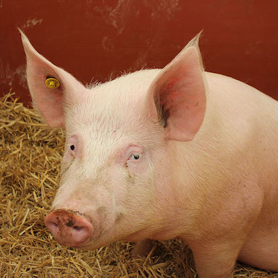
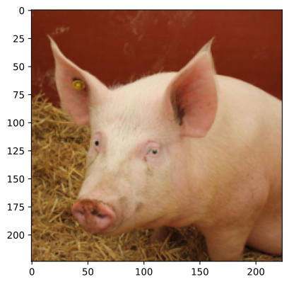
Wrap with ImageNet mean \((0.485, 0.456, 0.406)\) and std \((0.229, 0.224, 0.225)\). The executed notebook prints:
hog
Cross Entropy Loss: 0.00388, Expected probability: exp(-0.00388) = 0.996
The picture is a hog at probability 0.996. That is the starting point of both attacks.
pred = model(norm((x + delta).clip(0, 1)))
loss = -CrossEntropy(pred, y=341)
opt.step(); delta.data.clamp_(-epsilon, epsilon)
The notebook loss (negative CE) goes from about \(-0.015\) to about \(-17\). True-class probability collapses to \(1.0\times 10^{-7}\). The new top class is piggy_bank (719) at probability 0.996. The photograph still looks like a hog; \(50\delta+0.5\) is structured noise.
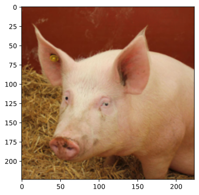
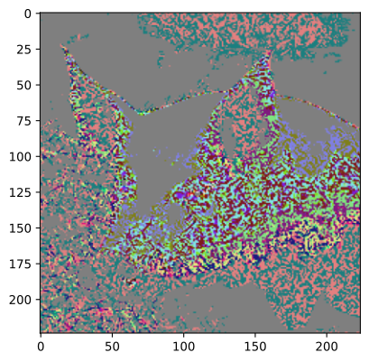
pred = model(norm((x + delta).clip(0, 1)))
loss = -CrossEntropy(pred, y=341) + CrossEntropy(pred, y=404)
# 100 SGD steps, lr=5e-3; clamp δ each step; then
# delta = ((x + delta).clip(0, 1) - x)
The same notebook then minimises that sum. The executed log runs through step 80: the loss falls from \(+24\) to about \(-35\), so hog is being driven down and airliner up. Each step still clamps \(\delta\) to \(2/255\); after the loop it rewrites \(\delta\leftarrow\mathrm{clip}(x+\delta,0,1)-x\) so the saved image is in gamut. The 2-D widget below is that second loop, with an \(\ell_\infty\) box you can see.
This page does not re-run ResNet-50 in the browser. The widget uses the notebook’s two objectives on a tiny differentiable classifier in the plane. Press Take 8 SGD steps once: untargeted should leave hog, targeted should enter airliner.
Norm balls miss transformations that people still recognise: a translated or rotated hog is a hog, and \(\lVert\delta\rVert_\infty\) may be huge. Detecting attacks by the distribution of \(\delta\) is possible in isolation and easy to circumvent: an attacker who knows the detector optimises a perturbation that looks typical and still fools \(f\). That cat-and-mouse continues in later lectures.