Compress. Reconstruct. Compare.
Why this mattersLearn useful image features without class labels.
Try thisFollow one image. Notice where its information is compressed.
 Input · 784 pixels
 Reconstruction
Visual example: a linear autoencoder (PCA). The notebook trains a neural autoencoder.
The training target is the input image itself. Digit labels are not needed.
What stops the network from simply copying every pixel?
The bottleneck has fewer values than the input. It forces the model to keep useful structure. A small code can lose fine detail.
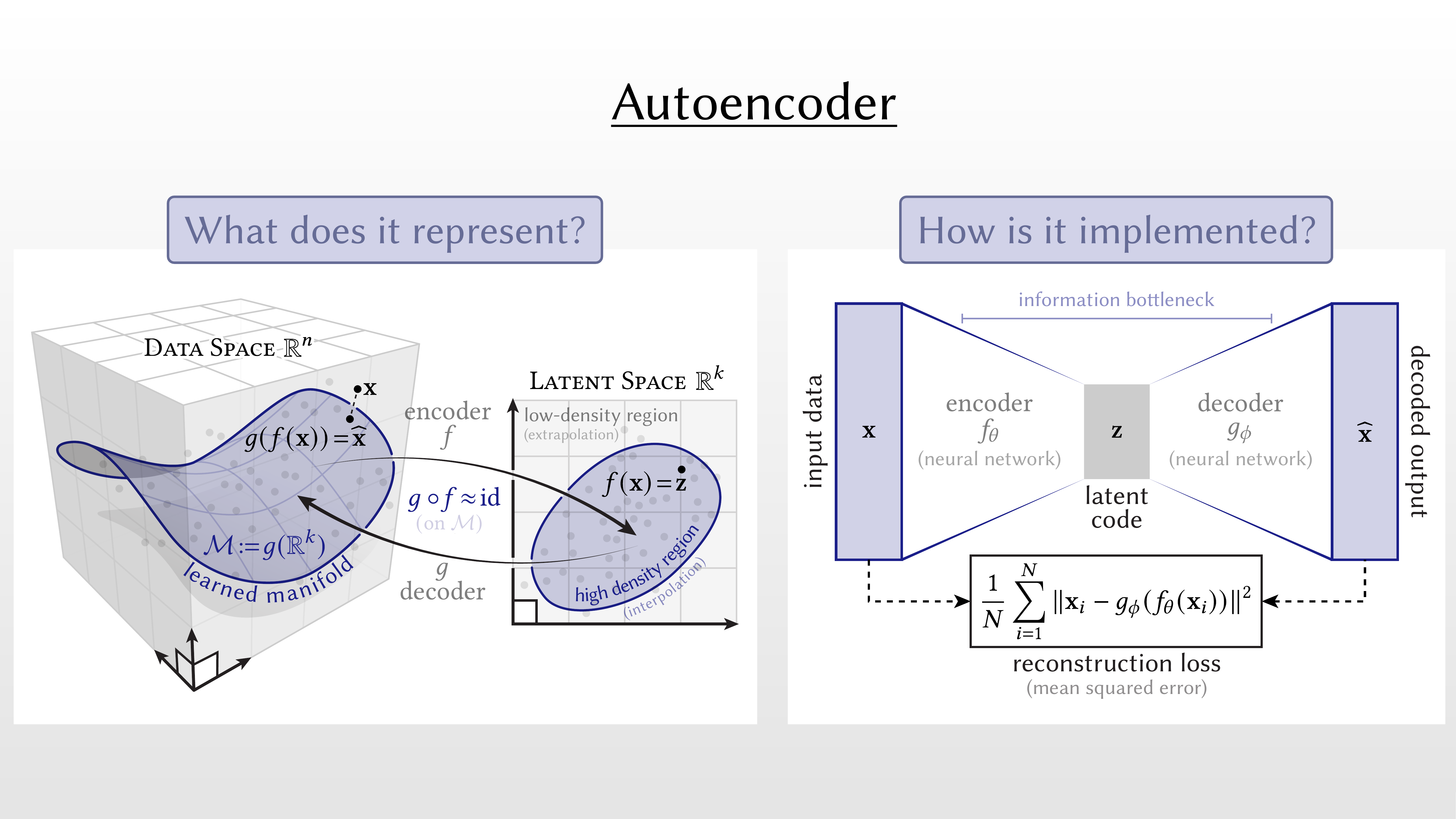
Two views of an autoencoder
Notebook source · 5 cells
Exact source and saved outputs. Python runs in Jupyter. Page controls use local teaching demos.
Cell 01 · Notebook text
# COMP90086 Workshop 9
Cell 02 · Notebook text
In this workshop, we will discuss generative models for images.

Table of Contents

- Autoencoders
    - Basic Autoencoder
    - Convolutional Autoencoder for Image Denoising
    - (Extra bonus) Convolutional Variational Autoencoder
- GANs
    - Play with GANs in your browser
    - DCGAN
Cell 03 · Python · import matplotlib.pyplot as plt
import matplotlib.pyplot as plt
import numpy as np
import tensorflow as tf
import os
import time

from tensorflow import keras
from tensorflow.keras import layers
from tensorflow.keras.models import Model

from IPython import display

print("TensorFlow version: ", tf.__version__)
Stored output
TensorFlow version: 2.17.0
Cell 04 · Notebook text
# 1. Autoencoders

Adapted from the Keras Blog and TensorFlow.org tutorials:
<table class="tfo-notebook-buttons" align="left">
    <td>
    <a target="_blank" href="https://blog.keras.io/building-autoencoders-in-keras.html">
    <img src="https://upload.wikimedia.org/wikipedia/commons/thumb/a/ae/Keras_logo.svg/240px-Keras_logo.svg.png" width=32/>
    View source on blog.keras.io</a>
  </td>
    <td>
    <a target="_blank" href="https://www.tensorflow.org/tutorials/generative/autoencoder">
    <img src="https://www.tensorflow.org/images/tf_logo_32px.png" />
    View source on TensorFlow.org</a>
  </td>
  <td>
    <a target="_blank" href="https://colab.research.google.com/github/tensorflow/docs/blob/master/site/en/tutorials/generative/autoencoder.ipynb">
    <img src="https://www.tensorflow.org/images/colab_logo_32px.png" />
    Run in Google Colab</a>
  </td>
  <td>
    <a target="_blank" href="https://github.com/tensorflow/docs/blob/master/site/en/tutorials/generative/autoencoder.ipynb">
    <img src="https://www.tensorflow.org/images/GitHub-Mark-32px.png" />
    View source on GitHub</a>
  </td>
</table>
Cell 05 · Notebook text
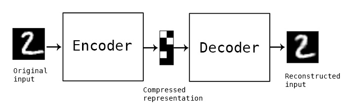
An autoencoder is a special type of neural network that is trained to copy its input to its output. For example, given an image of a handwritten digit, an autoencoder first encodes the image into a lower dimensional latent representation, then decodes the latent representation back to an image. An autoencoder learns to compress the data while minimizing the reconstruction error. 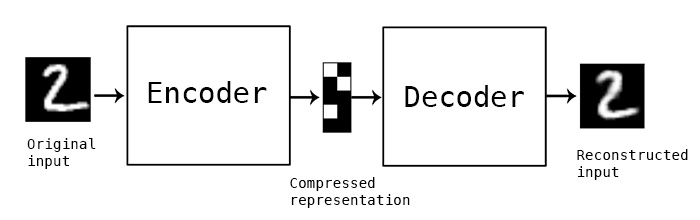 <center>Image source: the Keras Blog</center> We will introduce autoencoders with three examples: basic autoencoder, image denoising, and convolutional variational autoencoder.
What does the code represent?
Why this mattersUnderstand which images the decoder can produce.
Try thisSelect high and low density. Compare how much training evidence each region has.
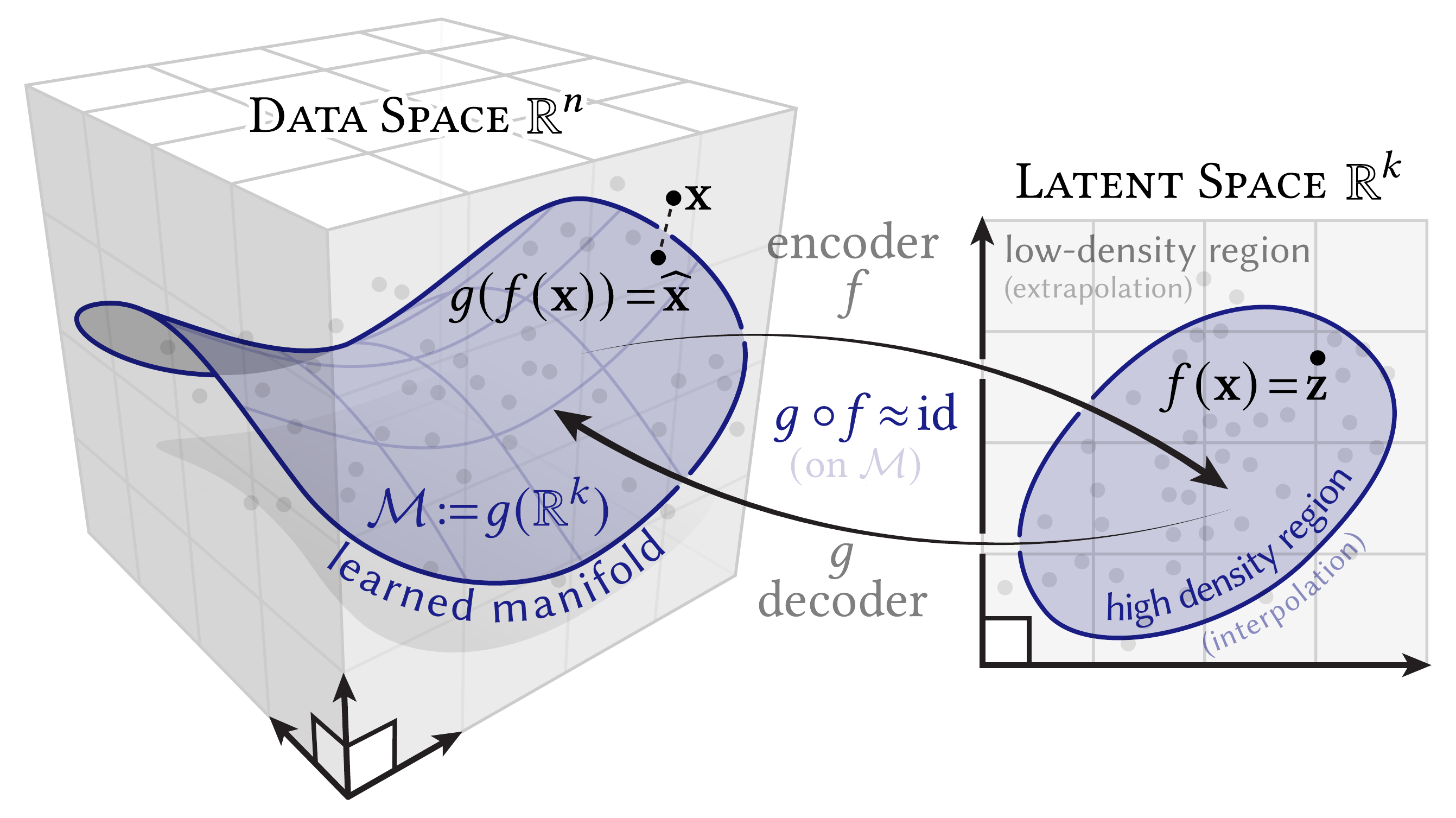
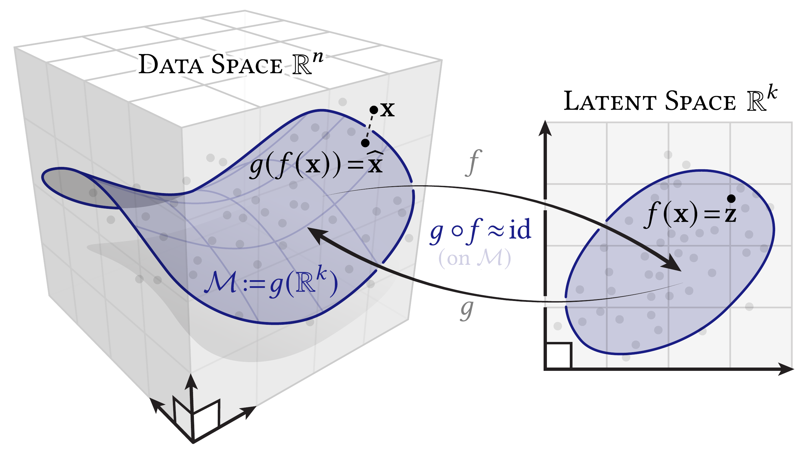
Select a label to explore the diagram. Figures: Keenan Crane, CC0.
The maps and their limits
Encoder: $z=f_\theta(x)$. Decoder: $\hat{x}=g_\phi(z)$.
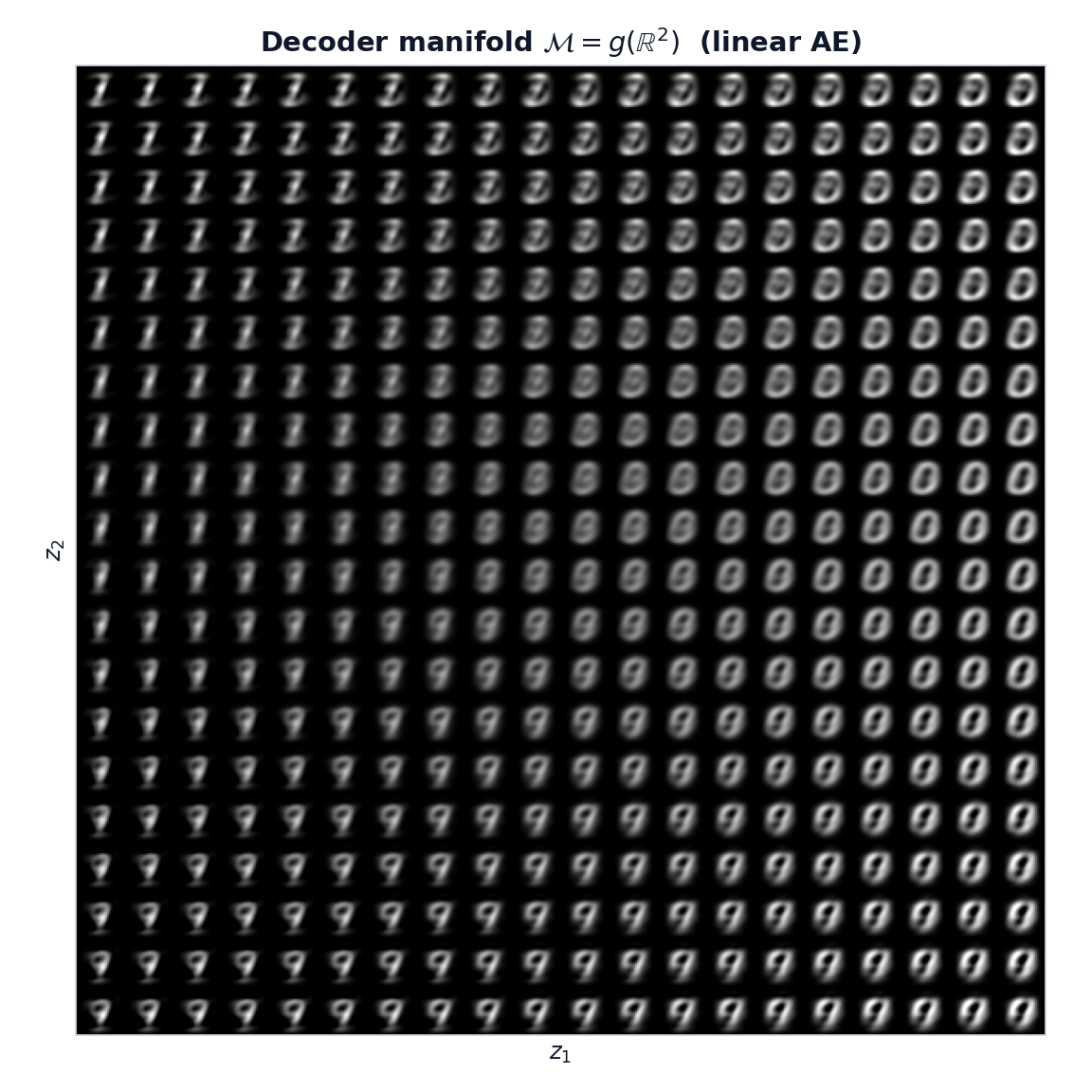
$$\mathcal M=g_\phi(\mathbb R^k),\qquad \dim(\mathcal M)\leq k$$Training encourages $g_\phi(f_\theta(x))\approx x$ on the data. It does not guarantee an identity map everywhere on $\mathcal M$.
The output lies on the decoder manifold. The input may not. Zero training loss alone does not prove overfitting; compare held-out results.
High and low density have no hard boundary. A basic autoencoder does not define a simple sampling distribution.
Why can a random latent code produce a poor image?
The decoder may never have seen nearby codes during training. Reconstruction training alone does not make all latent regions useful.
Prepare the digit images
Why this mattersGive the network consistent pixel values and shapes.
Try thisFollow one image from 28 × 28 pixels to a 784-value vector.
Setup and data code
import matplotlib.pyplot as plt
import numpy as np
import tensorflow as tf
import os
import time

from tensorflow import keras
from tensorflow.keras import layers
from tensorflow.keras.models import Model

from IPython import display

print("TensorFlow version: ", tf.__version__)# Since we only need images from the dataset to encode and decode,
# we won't use the labels.
(train_data, _), (test_data, test_labels) = keras.datasets.mnist.load_data()
# Normalize and reshape the data
train_data = train_data.astype('float32') / 255.
test_data = test_data.astype('float32') / 255.
x_train = train_data.reshape((len(train_data), np.prod(train_data.shape[1:])))
x_test = test_data.reshape((len(test_data), np.prod(test_data.shape[1:])))
print("train_images shape:", x_train.shape)
print("test_images shape:", x_test.shape)Why are the labels kept out of the training target?
The task is reconstruction. Each image supplies its own target. Labels only help us interpret the latent plot.
Notebook source · 3 cells
Exact source and saved outputs. Python runs in Jupyter. Page controls use local teaching demos.
Cell 06 · Notebook text
## Load the MNIST dataset and Prepare the data
We will train the basic autoencoder using the MNIST dataset.
MNIST is a dataset that consists of images of handwritten digits:
* the input data are images of handwritten digits (28×28 pixels with a single 8-bit channel)
* the target is a label in the set $\{0, 1, \ldots, 9\}$
The data is already split into training and test sets. The training set contains 60,000 instances and the test set contains 10,000 instances.Cell 07 · Notebook text
Let's prepare our input data. We're using MNIST digits. We load the data into NumPy arrays using a built-in function from Keras, and we're discarding the labels (since we're only interested in encoding/decoding the input images).
Cell 08 · Python · (train_data, _), (test_data, test_labels) = keras.datasets.mnist.load_
# Since we only need images from the dataset to encode and decode,
# we won't use the labels.
(train_data, _), (test_data, test_labels) = keras.datasets.mnist.load_data()

# Normalize and reshape the data
train_data = train_data.astype('float32') / 255.
test_data = test_data.astype('float32') / 255.

x_train = train_data.reshape((len(train_data), np.prod(train_data.shape[1:])))
x_test = test_data.reshape((len(test_data), np.prod(test_data.shape[1:])))

print("train_images shape:", x_train.shape)
print("test_images shape:", x_test.shape)Stored output
train_images shape: (60000, 784)
test_images shape: (10000, 784)
Train the basic autoencoder
Why this mattersCheck whether training improves reconstruction on held-out images.
Try thisPlay the loss chart. Compare the training and validation curves.
BCE and MSE
Why this formula? Use these losses to compare predicted pixels with target pixels. A smaller value means a closer reconstruction under that loss.
Both losses measure reconstruction error. This notebook uses BCE with sigmoid outputs.
$$\mathrm{BCE}=-\frac1D\sum_{d=1}^D[x_d\log\hat{x}_d+(1-x_d)\log(1-\hat{x}_d)]$$$$\mathrm{MSE}=\frac1D\sum_{d=1}^D(x_d-\hat{x}_d)^2$$$D=784$ pixels. BCE treats each pixel as a Bernoulli mean. MSE is the squared pixel error.
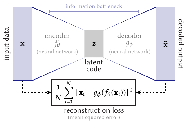
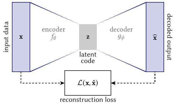
What do you pass as x and y in fit()?
Pass x_train twice. Use (x_test, x_test) for validation. Both notebook losses settle near 0.09.
Notebook source · 11 cells
Exact source and saved outputs. Python runs in Jupyter. Page controls use local teaching demos.
Cell 09 · Notebook text
## (1) Basic autoencoder

Let's start simple, with a single fully-connected neural layer as encoder and as decoder.


Define an autoencoder with two Dense layers: an `encoder`, which compresses the images into a 32 dimensional latent vector, and a `decoder`, that reconstructs the original image from the latent space.
Cell 10 · Python · latent_dim = 32 # 32 floats -> compression of factor 24.5, assuming t
# This is the size of our encoded representations
latent_dim = 32  # 32 floats -> compression of factor 24.5, assuming the input is 784 floats

# This is our input image
input_img = keras.Input(shape=(784,))
# "encoded" is the encoded representation of the input
encoded = layers.Dense(latent_dim, activation='relu')(input_img)
# "decoded" is the lossy reconstruction of the input
decoded = layers.Dense(784, activation='sigmoid')(encoded)

# This model maps an input to its reconstruction
autoencoder = keras.Model(input_img, decoded)
Cell 11 · Notebook text
Let's also create a separate encoder model:
Cell 12 · Python · encoder = keras.Model(input_img, encoded)
# This model maps an input to its encoded representation
encoder = keras.Model(input_img, encoded)
Cell 13 · Notebook text
As well as the decoder model:
Cell 14 · Python · encoded_input = keras.Input(shape=(latent_dim,))
# This is our encoded (32-dimensional) input
encoded_input = keras.Input(shape=(latent_dim,))
# Retrieve the last layer of the autoencoder model
decoder_layer = autoencoder.layers[-1]
# Create the decoder model
decoder = keras.Model(encoded_input, decoder_layer(encoded_input))
Cell 15 · Notebook text
Now let's train our autoencoder to reconstruct MNIST digits.

First, we'll configure our model to use a per-pixel binary crossentropy loss, and the Adam optimizer:
Cell 16 · Python · autoencoder.compile(optimizer='adam', loss='binary_crossentropy')
autoencoder.compile(optimizer='adam', loss='binary_crossentropy')Cell 17 · Notebook text
Now let's train our autoencoder for 20 epochs:
Cell 18 · Python · autoencoder.fit(x_train, x_train,
autoencoder.fit(x_train, x_train,
                epochs=20,
                batch_size=256,
                shuffle=True,
                validation_data=(x_test, x_test))
Stored output
Epoch 1/20
235/235 ━━━━━━━━━━━━━━━━━━━━ 1s 3ms/step - loss: 0.3786 - val_loss: 0.1932
Epoch 2/20
235/235 ━━━━━━━━━━━━━━━━━━━━ 1s 3ms/step - loss: 0.1828 - val_loss: 0.1548
Epoch 3/20
235/235 ━━━━━━━━━━━━━━━━━━━━ 1s 3ms/step - loss: 0.1506 - val_loss: 0.1345
Epoch 4/20
235/235 ━━━━━━━━━━━━━━━━━━━━ 1s 3ms/step - loss: 0.1324 - val_loss: 0.1215
Epoch 5/20
235/235 ━━━━━━━━━━━━━━━━━━━━ 1s 3ms/step - loss: 0.1209 - val_loss: 0.1131
Epoch 6/20
235/235 ━━━━━━━━━━━━━━━━━━━━ 1s 3ms/step - loss: 0.1133 - val_loss: 0.1076
Epoch 7/20
235/235 ━━━━━━━━━━━━━━━━━━━━ 1s 3ms/step - loss: 0.1079 - val_loss: 0.1037
Epoch 8/20
235/235 ━━━━━━━━━━━━━━━━━━━━ 1s 3ms/step - loss: 0.1041 - val_loss: 0.1006
Epoch 9/20
235/235 ━━━━━━━━━━━━━━━━━━━━ 1s 3ms/step - loss: 0.1013 - val_loss: 0.0984
Epoch 10/20
235/235 ━━━━━━━━━━━━━━━━━━━━ 1s 3ms/step - loss: 0.0993 - val_loss: 0.0968
Epoch 11/20
235/235 ━━━━━━━━━━━━━━━━━━━━ 1s 3ms/step - loss: 0.0979 - val_loss: 0.0957
Epoch 12/20
235/235 ━━━━━━━━━━━━━━━━━━━━ 1s 3ms/step - loss: 0.0970 - val_loss: 0.0951
Epoch 13/20
235/235 ━━━━━━━━━━━━━━━━━━━━ 1s 3ms/step - loss: 0.0963 - val_loss: 0.0947
Epoch 14/20
235/235 ━━━━━━━━━━━━━━━━━━━━ 1s 3ms/step - loss: 0.0959 - val_loss: 0.0943
Epoch 15/20
235/235 ━━━━━━━━━━━━━━━━━━━━ 1s 3ms/step - loss: 0.0955 - val_loss: 0.0941
Epoch 16/20
235/235 ━━━━━━━━━━━━━━━━━━━━ 1s 3ms/step - loss: 0.0953 - val_loss: 0.0939
Epoch 17/20
235/235 ━━━━━━━━━━━━━━━━━━━━ 1s 3ms/step - loss: 0.0950 - val_loss: 0.0938
Epoch 18/20
235/235 ━━━━━━━━━━━━━━━━━━━━ 1s 3ms/step - loss: 0.0950 - val_loss: 0.0936
Epoch 19/20
235/235 ━━━━━━━━━━━━━━━━━━━━ 1s 3ms/step - loss: 0.0950 - val_loss: 0.0936
Epoch 20/20
235/235 ━━━━━━━━━━━━━━━━━━━━ 1s 3ms/step - loss: 0.0948 - val_loss: 0.0935
<keras.src.callbacks.history.History at 0x30d6affd0>
Cell 19 · Notebook text
After 20 epochs, the autoencoder seems to reach a stable train/validation loss value of about 0.09. We can try to visualize the reconstructed inputs and the encoded representations.
Read the reconstructions and codes
Why this mattersCheck what the model preserves and how it groups similar inputs.
Try thisCompare original and reconstructed strokes. Then inspect nearby colours in t-SNE.
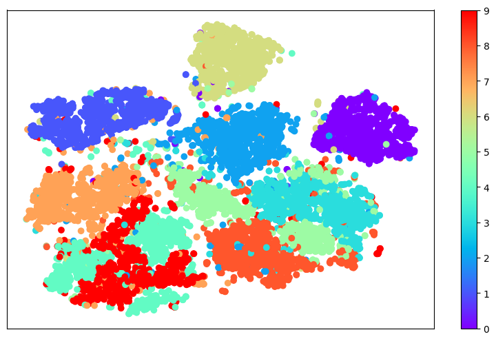
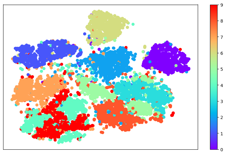
t-SNE is a view of the code, not the code itself. Large distances and cluster sizes can be misleading.
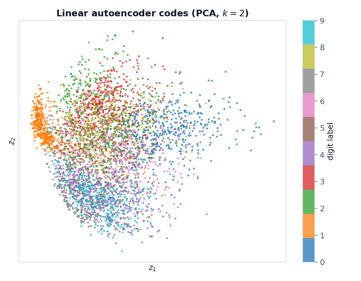
A linear baseline: PCA
A linear autoencoder trained with squared error can learn the PCA subspace. This result does not apply to every autoencoder loss.
Do overlapping colours mean the autoencoder failed?
No. Similar handwriting can share useful features. The loss rewards reconstruction, not class separation. Inspect the reconstructions and local neighbours too.
Notebook source · 7 cells
Exact source and saved outputs. Python runs in Jupyter. Page controls use local teaching demos.
Cell 20 · Python · encoded_imgs = encoder.predict(x_test)
# Encode and decode some digits
# Note that we take them from the *test* set
encoded_imgs = encoder.predict(x_test)
decoded_imgs = decoder.predict(encoded_imgs)
Stored output
313/313 ━━━━━━━━━━━━━━━━━━━━ 0s 261us/step
313/313 ━━━━━━━━━━━━━━━━━━━━ 0s 291us/step
Cell 21 · Notebook text
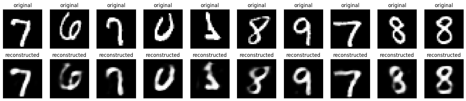
Define a `display` function to display ten random images.
Cell 22 · Python · def display(array1, array2):
def display(array1, array2):
    """
    Displays ten random images from each one of the supplied arrays.
    """

    n = 10 # How many digits we will display

    indices = np.random.randint(len(array1), size=n)
    images1 = array1[indices, :]
    images2 = array2[indices, :]

    plt.figure(figsize=(20, 4))
    for i, (image1, image2) in enumerate(zip(images1, images2)):
        # Display original
        ax = plt.subplot(2, n, i + 1)
        plt.imshow(image1.reshape(28, 28))
        plt.title("original")
        plt.gray()
        ax.get_xaxis().set_visible(False)
        ax.get_yaxis().set_visible(False)

        # Display reconstruction
        ax = plt.subplot(2, n, i + 1 + n)
        plt.imshow(image2.reshape(28, 28))
        plt.gray()
        plt.title("reconstructed")
        ax.get_xaxis().set_visible(False)
        ax.get_yaxis().set_visible(False)

    plt.show()
Cell 23 · Python · display(x_test, decoded_imgs)
# Display the test data and the reconstructed results
display(x_test, decoded_imgs)
Stored output
<Figure size 2000x400 with 20 Axes>
Cell 24 · Notebook text
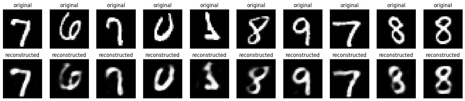
Here's what we get. The top row is the original digits, and the bottom row is the reconstructed digits. The autoencoder is able to recreate digits quite accurately, although there is some information loss.
Cell 25 · Notebook text
### Visualise the latent space

The autoencoder has learned a latent representation of the images, which is a compressed representation (in this case, just 32 values) that represent the variation in the MNIST images. We can use [TSNE](https://scikit-learn.org/stable/modules/generated/sklearn.manifold.TSNE.html) to visualise the latent space. This is a form of dimensionality-reduction that tries to preserve the distances between points as much as possible -- points that are nearby in the latent space will be nearby in the 2D plot. Different digits are shown in different colours.
Cell 26 · Python · from sklearn.manifold import TSNE
from sklearn.manifold import TSNE

# using t-SNE to visualise the latent space
tsne = TSNE(n_components=2)
X_tsne = tsne.fit_transform(encoded_imgs)

plt.figure(figsize=(10, 6))
plt.scatter(X_tsne[:,0], X_tsne[:,1], c= test_labels, cmap='rainbow')
plt.colorbar()
plt.xticks([])
plt.yticks([])
plt.show()
Stored output
<Figure size 1000x600 with 2 Axes>
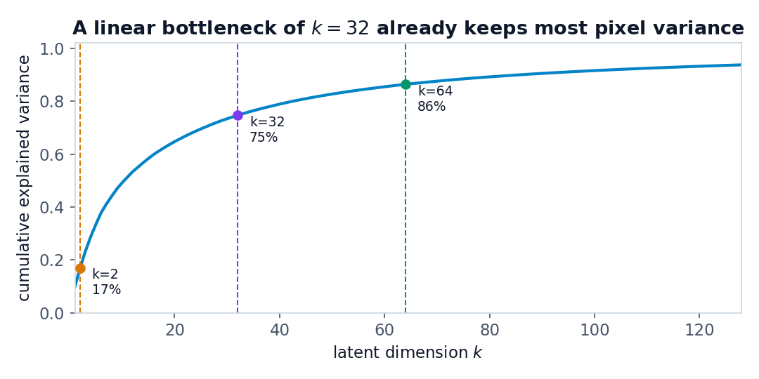
How small can the code be?
Why this mattersChoose a code size that balances detail and compression.
Try thisReduce k. Predict which stroke details will disappear.
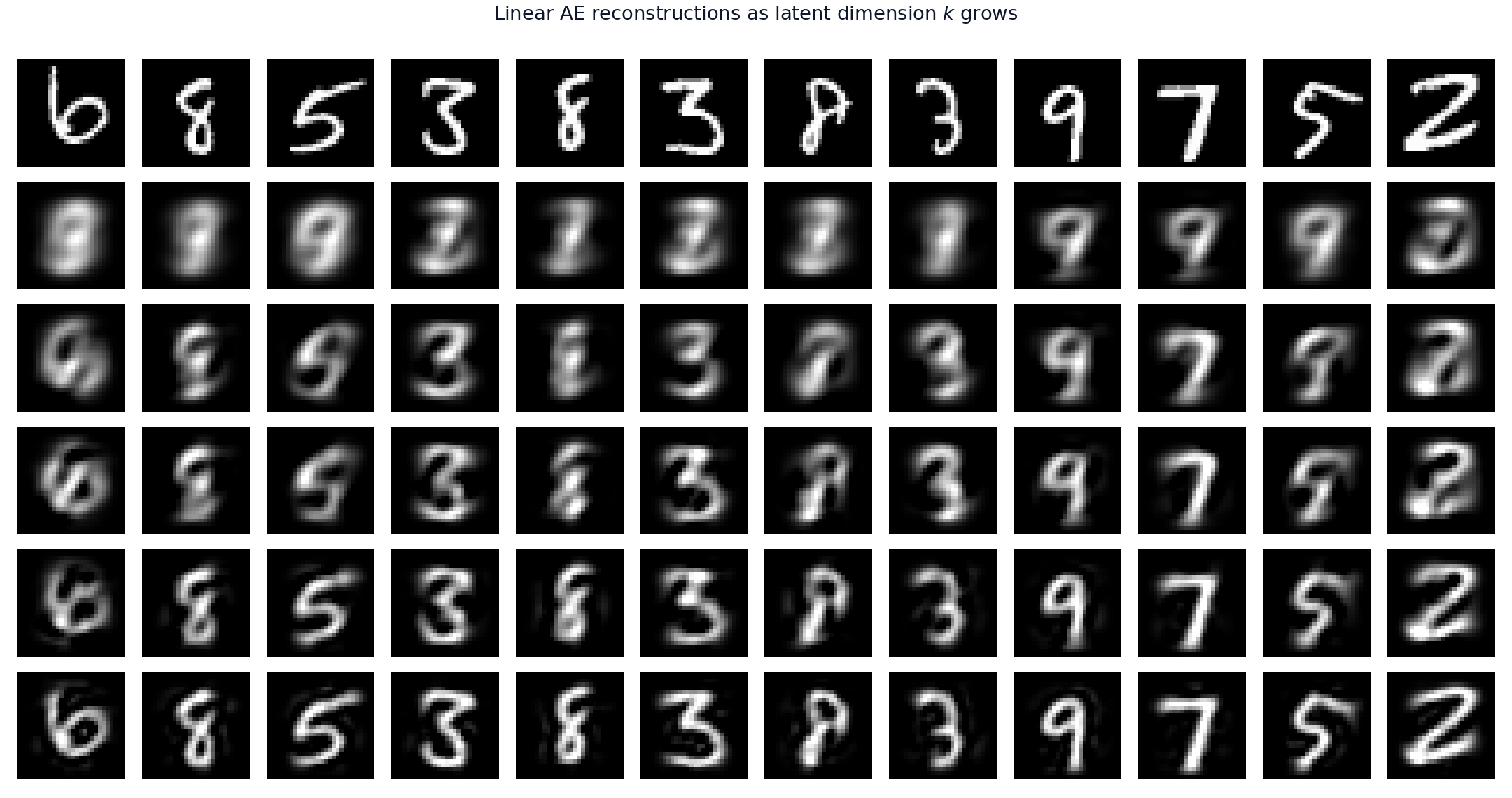
Change k below. Watch the reconstructed digit and its pixel error. All values in this visual come from PCA.
The notebook uses k = 32. This interactive example uses PCA.
How does k affect reconstruction and digit clusters? Why?
Small k: less room for detail. Reconstructions often blur. Codes for similar shapes may overlap.
Large k: more capacity and less compression. Better reconstruction is possible, but class separation is not guaranteed.
Look for: 4 and 9, or 3, 5, and 8. Their strokes can look similar. Check your own plot; the pattern can change.
Why: the loss compares pixels. It does not use class labels. At k = 32, the value-count ratio is 784 / 32 = 24.5. This is not a file-compression ratio.
Teaching answer. The solution notebook leaves this exercise cell empty.
Compare all five PCA results
Notebook source · 2 cells
Exact source and saved outputs. Python runs in Jupyter. Page controls use local teaching demos.
Cell 27 · Notebook text
### Exercise 1: Investigate the latent space representation of MNIST digits

Try changing the size of the latent space. How does this affect the reconstruction results and the organisation of digits in the latent space? Why?

You may notice the representations of different digits overlap in the latent space, particularly when the latent space is very small. Which digits cluster together in the latent space? Do these clusters make sense?
Cell 28 · Python · Exercise space
# Empty exercise cell in the source notebook.Add noise. Keep the target clean.
Why this mattersCreate training pairs that teach the model to remove noise.
Try thisIncrease the noise. Notice that the clean target stays fixed.
Left: clean $x$. Middle: noisy $\tilde{x}$. Right: the target is still $x$, not $\tilde{x}$.
Noise equation
def noise(array):
    """
    Adds random noise to each image in the supplied array.
    """

    noise_factor = 0.4
    noisy_array = array + noise_factor * np.random.normal(
        loc=0.0, scale=1.0, size=array.shape
    )

    return np.clip(noisy_array, 0.0, 1.0)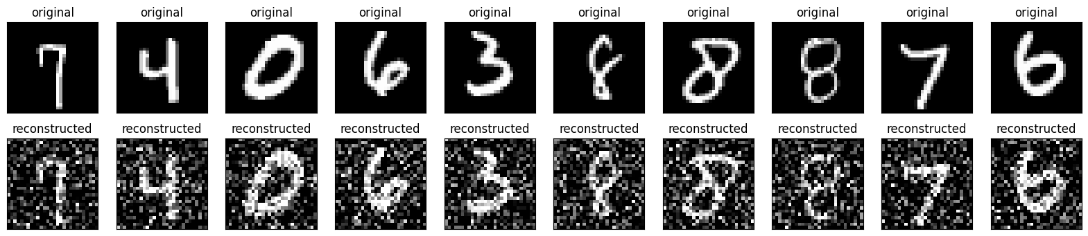
If the input is noisy, should the target also be noisy?
No. Keep the clean image as the target. Otherwise, the network learns to reproduce noise.
Notebook source · 4 cells
Exact source and saved outputs. Python runs in Jupyter. Page controls use local teaching demos.
Cell 29 · Notebook text
## (2) Convolutional autoencoder for image denoising

An autoencoder can also be trained to remove noise from images. In the following section, you will create a noisy version of the MNIST dataset by applying random noise to each image. You will then train a deep convolutional autoencoder for image denoising, mapping noisy digits images from the MNIST dataset to clean digits images.

Below we define a `noise` function to add random noise to each image.
Cell 30 · Python · def noise(array):
def noise(array):
    """
    Adds random noise to each image in the supplied array.
    """

    noise_factor = 0.4
    noisy_array = array + noise_factor * np.random.normal(
        loc=0.0, scale=1.0, size=array.shape
    )

    return np.clip(noisy_array, 0.0, 1.0)
Cell 31 · Notebook text
Let's reuse the dataset we loaded earlier.
Cell 32 · Python · x_train = np.reshape(train_data, (len(train_data), 28, 28, 1))
# Reshape the data
x_train = np.reshape(train_data, (len(train_data), 28, 28, 1))
x_test = np.reshape(test_data, (len(test_data), 28, 28, 1))

# Create a copy of the data with added noise
noisy_train_data = noise(x_train)
noisy_test_data = noise(x_test)

# Display the train data and a version of it with added noise
display(x_train, noisy_train_data)
Stored output
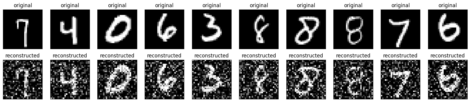
<Figure size 2000x400 with 20 Axes>
Learn to remove the noise
Why this mattersRecover image structure from a corrupted input.
Try thisFollow the feature-map sizes. Compare noisy inputs with the clean estimates.
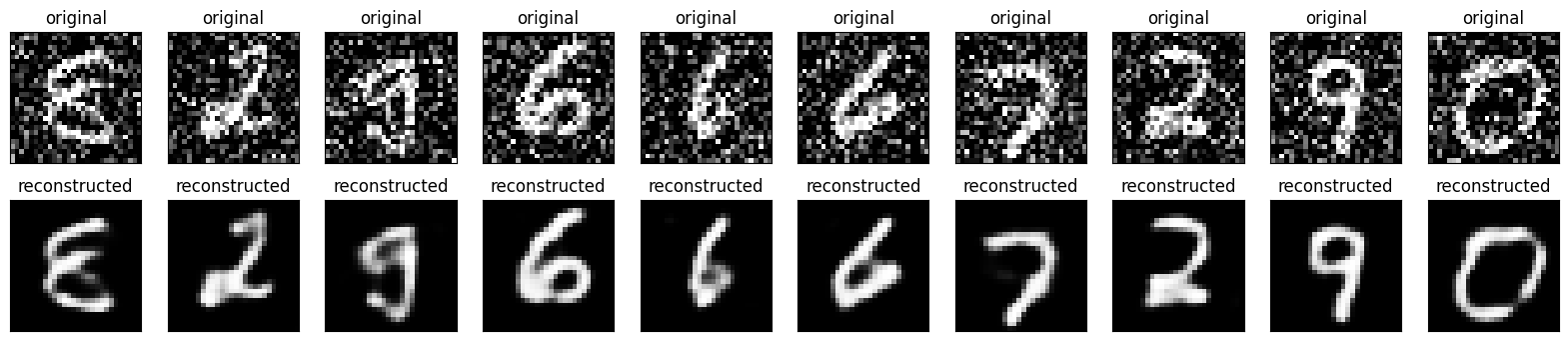
Fit noisy_train_data → x_train. Validate noisy_test_data → x_test. Training may take time; use the stored result to discuss the outcome.
How does this task differ from the basic autoencoder?
The basic model maps clean → clean. The denoising model maps noisy → clean. Both minimise reconstruction loss. Denoising encourages features that survive input noise.
Notebook source · 5 cells
Exact source and saved outputs. Python runs in Jupyter. Page controls use local teaching demos.
Cell 33 · Notebook text
Can our autoencoder learn to recover the original digits? Let's find out.

**Build the autoencoder.**

Compared to the previous convolutional autoencoder, in order to improve the quality of the reconstructed, we'll use a slightly different model with more filters per layer:

We are going to use the Functional API to build our convolutional autoencoder.
Cell 34 · Python · input = layers.Input(shape=(28, 28, 1))
input = layers.Input(shape=(28, 28, 1))

# Encoder
x = layers.Conv2D(32, (3, 3), activation="relu", padding="same")(input)
x = layers.MaxPooling2D((2, 2), padding="same")(x)
x = layers.Conv2D(32, (3, 3), activation="relu", padding="same")(x)
x = layers.MaxPooling2D((2, 2), padding="same")(x)

# Decoder
x = layers.Conv2DTranspose(32, (3, 3), strides=2, activation="relu", padding="same")(x)
x = layers.Conv2DTranspose(32, (3, 3), strides=2, activation="relu", padding="same")(x)
x = layers.Conv2D(1, (3, 3), activation="sigmoid", padding="same")(x)

# Autoencoder
autoencoder = Model(input, x)
autoencoder.compile(optimizer="adam", loss="binary_crossentropy")
autoencoder.summary()
Stored output
Model: "functional_3"
┏━━━━━━━━━━━━━━━━━━━━━━━━━━━━━━━━━┳━━━━━━━━━━━━━━━━━━━━━━━━┳━━━━━━━━━━━━━━━┓
┃ Layer (type)                    ┃ Output Shape           ┃       Param # ┃
┡━━━━━━━━━━━━━━━━━━━━━━━━━━━━━━━━━╇━━━━━━━━━━━━━━━━━━━━━━━━╇━━━━━━━━━━━━━━━┩
│ input_layer_2 (InputLayer)      │ (None, 28, 28, 1)      │             0 │
├─────────────────────────────────┼────────────────────────┼───────────────┤
│ conv2d (Conv2D)                 │ (None, 28, 28, 32)     │           320 │
├─────────────────────────────────┼────────────────────────┼───────────────┤
│ max_pooling2d (MaxPooling2D)    │ (None, 14, 14, 32)     │             0 │
├─────────────────────────────────┼────────────────────────┼───────────────┤
│ conv2d_1 (Conv2D)               │ (None, 14, 14, 32)     │         9,248 │
├─────────────────────────────────┼────────────────────────┼───────────────┤
│ max_pooling2d_1 (MaxPooling2D)  │ (None, 7, 7, 32)       │             0 │
├─────────────────────────────────┼────────────────────────┼───────────────┤
│ conv2d_transpose                │ (None, 14, 14, 32)     │         9,248 │
│ (Conv2DTranspose)               │                        │               │
├─────────────────────────────────┼────────────────────────┼───────────────┤
│ conv2d_transpose_1              │ (None, 28, 28, 32)     │         9,248 │
│ (Conv2DTranspose)               │                        │               │
├─────────────────────────────────┼────────────────────────┼───────────────┤
│ conv2d_2 (Conv2D)               │ (None, 28, 28, 1)      │           289 │
└─────────────────────────────────┴────────────────────────┴───────────────┘
Total params: 28,353 (110.75 KB)
Trainable params: 28,353 (110.75 KB)
Non-trainable params: 0 (0.00 B)
Cell 35 · Notebook text
Now we can train our autoencoder using the noisy data as our input and the clean data as our target. We want our autoencoder to learn how to denoise the images.

**This may take a while, please refer to your tutor's demonstration of the results during the workshop.**
Cell 36 · Python · autoencoder.fit(
autoencoder.fit(
    x=noisy_train_data,
    y=x_train,
    epochs=2,
    batch_size=128,
    shuffle=True,
    validation_data=(noisy_test_data, x_test),
)
Stored output
Epoch 1/2
469/469 ━━━━━━━━━━━━━━━━━━━━ 16s 33ms/step - loss: 0.2862 - val_loss: 0.1020
Epoch 2/2
469/469 ━━━━━━━━━━━━━━━━━━━━ 16s 35ms/step - loss: 0.1013 - val_loss: 0.0970
<keras.src.callbacks.history.History at 0x36391ac70>
Cell 37 · Python · predictions = autoencoder.predict(noisy_test_data)
predictions = autoencoder.predict(noisy_test_data)
display(noisy_test_data, predictions)
Stored output
313/313 ━━━━━━━━━━━━━━━━━━━━ 2s 5ms/step
<Figure size 2000x400 with 20 Axes>
Give latent space a sampling rule
Why this mattersGive the decoder a useful rule for drawing new latent codes.
Try thisDraw several codes. Look for samples far from the example training codes.
The prior lands in a hole. $g$ must extrapolate.
The same prior now hits the cloud. $g$ interpolates.
Schematic codes, not trained model outputs. The circle marks a typical region of a Gaussian prior. The Gaussian also has mass outside it.
Regularisation supports sampling. It does not guarantee a good image at every latent point.
Where does a new code come from when a VAE generates an image?
Sample it from the prior, usually N(0, I). Then decode it. An input image is not needed for this generation step.
Notebook bonus and optional tutorials
The notebook introduces the idea and links to a standalone example. It does not include VAE training cells.
Notebook source · 2 cells
Exact source and saved outputs. Python runs in Jupyter. Page controls use local teaching demos.
Cell 38 · Notebook text
## (3) Extra bonus: Convolutional Variational Autoencoder
Cell 39 · Notebook text
Variational autoencoders are a slightly more modern and interesting take on autoencoding.

What is a variational autoencoder? It's a type of autoencoder with added constraints on the encoded representations being learned. More precisely, it is an autoencoder that learns a latent variable model for its input data. So instead of letting your neural network learn an arbitrary function, you are learning the parameters of a probability distribution modeling your data. If you sample points from this distribution, you can generate new input data samples: a VAE is a "generative model".

Because a VAE is a more complex example, your could refer to the standalone script below:

<table class="tfo-notebook-buttons" align="left">
  <td>
    <a target="_blank" href="https://www.tensorflow.org/tutorials/generative/cvae">
    <img src="https://www.tensorflow.org/images/tf_logo_32px.png" />
    View on TensorFlow.org</a>
  </td>
  <td>
    <a target="_blank" href="https://colab.research.google.com/github/tensorflow/docs/blob/master/site/en/tutorials/generative/cvae.ipynb">
    <img src="https://www.tensorflow.org/images/colab_logo_32px.png" />
    Run in Google Colab</a>
  </td>

</table>Sample without breaking the gradient
Why this mattersLearn distribution parameters while still sampling random codes.
Try thisMove the mean or spread. Compare the sampled code, decoded image, and KL cost.
Move the mean and variance. Resample independent noise. The output uses a two-component PCA decoder.
A real PCA decoder maps the two coordinates to pixels. Each coordinate is scaled by its training standard deviation. This is not a trained VAE.
Dashed $=p(z)$. Solid $=q_\phi(z\mid x)$. KL is smallest when μ = 0 and σ = 1. Moving away from that point raises KL.
The same facts as formulas
Why this formula? Reconstruction keeps the output close to the input. KL keeps the encoded distribution close to the prior so sampling is useful.
From the notebook (Keras / Chollet): a VAE learns the parameters of a distribution on the latent space, not an arbitrary code. Sample that distribution, then decode.
$$q_\phi(z\mid x)=\mathcal{N}\bigl(\mu_\phi(x),\,\mathrm{diag}\,\sigma_\phi^2(x)\bigr)$$ $$z=\mu_\phi(x)+\sigma_\phi(x)\odot\varepsilon,\qquad \varepsilon\sim\mathcal{N}(0,I)$$ $$\mathcal{L}_{\mathrm{VAE}}=\underbrace{-\mathbb{E}_{q_\phi(z\mid x)}[\log p_\theta(x\mid z)]}_{\text{reconstruction}}+\underbrace{D_{\mathrm{KL}}\bigl(q_\phi(z\mid x)\,\|\,p(z)\bigr)}_{\text{regulariser}}$$ $$D_{\mathrm{KL}}=\frac{1}{2}\bigl(\mu^2+\sigma^2-\log\sigma^2-1\bigr)$$Which values minimise the KL term in the one-dimensional example?
μ = 0 and σ = 1. This matches the standard normal prior. A very small σ also incurs a KL cost.
Generate. Judge. Improve.
Why this mattersLearn to generate images from feedback rather than pixel targets.
Try thisPlay the game, then select mode collapse. Check how much of the data is covered.
Teal: real data. Orange: generated points. This is a teaching simulation, not a trained network. Play, then try mode collapse.
Can generated images look good while the model performs poorly?
Yes. A generator can repeat a few convincing images. High quality does not imply high diversity. Try “Mode collapse” in the simulation.
GAN Lab and model comparison
Open GAN Lab for a separate live training tool.
AE: reconstruct an input. VAE: reconstruct and sample a prior. GAN: generate from noise using a learned discriminator.
VAEs can produce softer images. GANs can produce fine detail, but training may be unstable. These are common tendencies, not fixed rules.
Notebook source · 4 cells
Exact source and saved outputs. Python runs in Jupyter. Page controls use local teaching demos.
Cell 40 · Notebook text
# 2. Generative Adversarial Networks (GANs)
Cell 41 · Notebook text
## (1) Warm-up [Play with GANs in your browser!](https://poloclub.github.io/ganlab/)
Cell 42 · Notebook text
### GANs, Autoencoders and VAEs
Generative adversarial networks (GANs) are algorithmic architectures that use two neural networks, pitting one against the other (thus the “adversarial”) in order to generate new, synthetic instances of data that can pass for real data. They are used widely in image generation, video generation and voice generation.

It may be useful to compare generative adversarial networks to other neural networks, such as autoencoders and variational autoencoders.

Autoencoders encode input data as vectors. They create a hidden, or compressed, representation of the raw data. They are useful in dimensionality reduction; that is, the vector serving as a hidden representation compresses the raw data into a smaller number of salient dimensions. Autoencoders can be paired with a so-called decoder, which allows you to reconstruct input data based on its hidden representation.

Variational autoencoders are generative algorithm that add an additional constraint to encoding the input data, namely that the hidden representations are normalized. Variational autoencoders are capable of both compressing data like an autoencoder and synthesizing data like a GAN. However, while GANs generate data in fine, granular detail, images generated by VAEs tend to be more blurred.

(Source of the above introduction: [Pathmind](https://wiki.pathmind.com/generative-adversarial-network-gan))
Cell 43 · Notebook text
## (2) DCGAN

We will introduce how to generate images of handwritten digits using a [Deep Convolutional Generative Adversarial Network](https://arxiv.org/abs/1511.06434) (DCGAN). We will still use the MNIST dataset to train the generator and the discriminator. The generator will generate handwritten digits resembling the MNIST data.

Adapted from TensorFlow.org tutorials:
<table class="tfo-notebook-buttons" align="left">
  <td>
    <a target="_blank" href="https://www.tensorflow.org/tutorials/generative/dcgan">
    <img src="https://www.tensorflow.org/images/tf_logo_32px.png" />
    View source on TensorFlow.org</a>
  </td>
  <td>
    <a target="_blank" href="https://colab.research.google.com/github/tensorflow/docs/blob/master/site/en/tutorials/generative/dcgan.ipynb">
    <img src="https://www.tensorflow.org/images/colab_logo_32px.png" />
    Run in Google Colab</a>
  </td>

</table>Prepare images for DCGAN
Why this mattersStop the discriminator from relying on a simple pixel-scale mismatch.
Try thisMove the pixel slider. Compare the AE range with the GAN range.
Why must real and generated images use the same range?
Otherwise, the discriminator can use a scale mismatch to separate them. It may learn little about digit structure.
Notebook source · 3 cells
Exact source and saved outputs. Python runs in Jupyter. Page controls use local teaching demos.
Cell 44 · Notebook text
### Load and prepare the dataset

Let's reimport the dataset to omit the modifications made earlier.
Cell 45 · Python · (x_train, _), (x_test, _) = tf.keras.datasets.mnist.load_data()
(x_train, _), (x_test, _) = tf.keras.datasets.mnist.load_data()
x_train = x_train.reshape(x_train.shape[0], 28, 28, 1).astype('float32')
x_train = (x_train - 127.5) / 127.5  # Normalize the images to [-1, 1]

x_test = x_test.reshape(x_test.shape[0], 28, 28, 1).astype('float32')
x_test = (x_test - 127.5) / 127.5  # Normalize the images to [-1, 1]

print("train_images shape:", x_train.shape)
print("test_images shape:", x_test.shape)
Stored output
train_images shape: (60000, 28, 28, 1)
test_images shape: (10000, 28, 28, 1)
Cell 46 · Python · BUFFER_SIZE = 60000
BUFFER_SIZE = 60000
BATCH_SIZE = 256

# Batch and shuffle the data
train_dataset = tf.data.Dataset.from_tensor_slices(x_train).shuffle(BUFFER_SIZE).batch(BATCH_SIZE)Build the generator and discriminator
Why this mattersSee how noise becomes an image, and an image becomes a score.
Try thisStep through both networks. Track width, height, and channels.
Before training
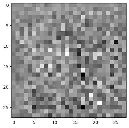
The untrained discriminator returns a score near zero. That score is not a probability.
Why does the discriminator end with one value?
It makes a binary decision: real or generated. It does not classify the digit as 0–9.
Notebook source · 9 cells
Exact source and saved outputs. Python runs in Jupyter. Page controls use local teaching demos.
Cell 47 · Notebook text
### Create the models

A GAN is made of two parts: a "generator" model that maps points in the latent space to points in image space, a "discriminator" model, a classifier that can tell the difference between real images (from the training dataset) and fake images (the output of the generator network).

<img style="float: ;" src="https://www.tensorflow.org/images/gan/dcgan.gif" width=600 height=500>
<center>(Image courtesy: tensorflow.org)</center>
Cell 48 · Notebook text
A GAN training loop looks like this:

- (1) Train the generator.
    - Sample random points in the latent space.
    - Turn the points into fake images via the "generator" network.
    - Get a batch of real images and combine them with the generated images.
    - Train the "generator" model to "fool" the discriminator and classify the fake images as real.

- (2) Train the discriminator.
    - Sample a batch of random points in the latent space.
    - Turn the points into fake images via the "generator" model.
    - Get a batch of real images and combine them with the generated images.
    - Train the "discriminator" model to classify generated vs. real images.

Let's implement this training loop.

#### The Generator

The generator uses `tf.keras.layers.Conv2DTranspose` (upsampling) layers to produce an image from a seed (random noise). Start with a `Dense` layer that takes this seed as input, then upsample several times until you reach the desired image size of 28x28x1. Notice the `tf.keras.layers.LeakyReLU` activation for each layer, except the output layer which uses tanh.
Cell 49 · Python · def make_generator_model():
def make_generator_model():
    model = tf.keras.Sequential()
    model.add(layers.Dense(7*7*256, use_bias=False, input_shape=(100,)))
    model.add(layers.BatchNormalization())
    model.add(layers.LeakyReLU())

    model.add(layers.Reshape((7, 7, 256)))
    assert model.output_shape == (None, 7, 7, 256)  # Note: None is the batch size

    model.add(layers.Conv2DTranspose(128, (5, 5), strides=(1, 1), padding='same', use_bias=False))
    assert model.output_shape == (None, 7, 7, 128)
    model.add(layers.BatchNormalization())
    model.add(layers.LeakyReLU())

    model.add(layers.Conv2DTranspose(64, (5, 5), strides=(2, 2), padding='same', use_bias=False))
    assert model.output_shape == (None, 14, 14, 64)
    model.add(layers.BatchNormalization())
    model.add(layers.LeakyReLU())

    model.add(layers.Conv2DTranspose(1, (5, 5), strides=(2, 2), padding='same', use_bias=False, activation='tanh'))
    assert model.output_shape == (None, 28, 28, 1)

    return model
Cell 50 · Notebook text
Use the (as yet untrained) generator to create an image.
Cell 51 · Python · generator = make_generator_model()
generator = make_generator_model()

noise = tf.random.normal([1, 100])
generated_image = generator(noise, training=False)

plt.imshow(generated_image[0, :, :, 0], cmap='gray')
Stored output
/Users/thixuanmayl/anaconda3/envs/py39/lib/python3.9/site-packages/keras/src/layers/core/dense.py:87: UserWarning: Do not pass an `input_shape`/`input_dim` argument to a layer. When using Sequential models, prefer using an `Input(shape)` object as the first layer in the model instead.
  super().__init__(activity_regularizer=activity_regularizer, **kwargs)
<matplotlib.image.AxesImage at 0x3637e7b50>
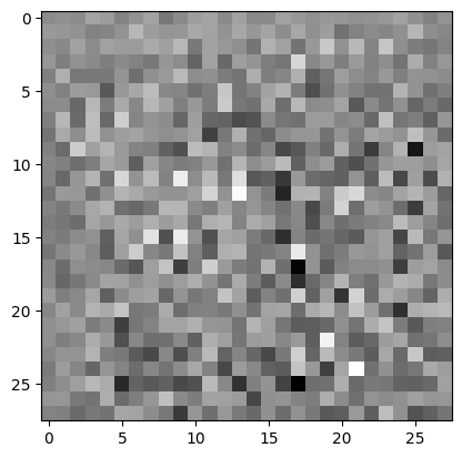
<Figure size 640x480 with 1 Axes>
Cell 52 · Notebook text
#### The Discriminator
Then, create the discriminator meant to classify fake vs real digits. The discriminator is a CNN-based image classifier.
Cell 53 · Python · def make_discriminator_model():
def make_discriminator_model():
    model = tf.keras.Sequential()
    model.add(layers.Conv2D(64, (5, 5), strides=(2, 2), padding='same',
                                     input_shape=[28, 28, 1]))
    model.add(layers.LeakyReLU())
    model.add(layers.Dropout(0.3))

    model.add(layers.Conv2D(128, (5, 5), strides=(2, 2), padding='same'))
    model.add(layers.LeakyReLU())
    model.add(layers.Dropout(0.3))

    model.add(layers.Flatten())
    model.add(layers.Dense(1))

    return model
Cell 54 · Notebook text
Use the (as yet untrained) discriminator to classify the generated images as real or fake. The model will be trained to output positive values for real images, and negative values for fake images.
Cell 55 · Python · discriminator = make_discriminator_model()
discriminator = make_discriminator_model()
decision = discriminator(generated_image)
print (decision)
Stored output
tf.Tensor([[-0.00164244]], shape=(1, 1), dtype=float32)
/Users/thixuanmayl/anaconda3/envs/py39/lib/python3.9/site-packages/keras/src/layers/convolutional/base_conv.py:107: UserWarning: Do not pass an `input_shape`/`input_dim` argument to a layer. When using Sequential models, prefer using an `Input(shape)` object as the first layer in the model instead.
  super().__init__(activity_regularizer=activity_regularizer, **kwargs)
Follow one training step
Why this mattersGive each network a training signal that matches its task.
Try thisCompare the fake-image target in the generator loss and discriminator loss.
Separate real from fake
Real → 1
Generated → 0
Make generated images pass
Generated → 1
Update G through D
Losses and the GAN objective
Why this formula? These losses tell each network which direction to improve. D learns to separate real and fake; G learns to make fakes pass.
$$L_D=\mathrm{BCE}(1,D(x))+\mathrm{BCE}(0,D(G(z)))$$$$L_G=\mathrm{BCE}(1,D(G(z)))$$These BCE calls use from_logits=True. The generator uses the non-saturating loss.
In the original minimax objective below, D denotes a probability:
$$\min_G\max_D\;\mathbb E_x[\log D(x)]+\mathbb E_z[\log(1-D(G(z)))]$$Why use target 1 for fake images in the generator loss?
The generator wants its images to be scored as real. The discriminator still uses target 0 when learning to identify those images as fake.
Notebook source · 11 cells
Exact source and saved outputs. Python runs in Jupyter. Page controls use local teaching demos.
Cell 56 · Notebook text
#### Define the loss and optimizers
Define loss functions and optimizers for both models.
Cell 57 · Python · cross_entropy = tf.keras.losses.BinaryCrossentropy(from_logits=True)
# This method returns a helper function to compute cross entropy loss
cross_entropy = tf.keras.losses.BinaryCrossentropy(from_logits=True)
Cell 58 · Notebook text
Discriminator loss

This method quantifies how well the discriminator is able to distinguish real images from fakes. It compares the discriminator's predictions on real images to an array of 1s, and the discriminator's predictions on fake (generated) images to an array of 0s.
Cell 59 · Python · def discriminator_loss(real_output, fake_output):
def discriminator_loss(real_output, fake_output):
    real_loss = cross_entropy(tf.ones_like(real_output), real_output)
    fake_loss = cross_entropy(tf.zeros_like(fake_output), fake_output)
    total_loss = real_loss + fake_loss
    return total_loss
Cell 60 · Notebook text
Generator loss

The generator's loss quantifies how well it was able to trick the discriminator. Intuitively, if the generator is performing well, the discriminator will classify the fake images as real (or 1). Here, compare the discriminators decisions on the generated images to an array of 1s.
Cell 61 · Python · def generator_loss(fake_output):
def generator_loss(fake_output):
    return cross_entropy(tf.ones_like(fake_output), fake_output)
Cell 62 · Notebook text
The discriminator and the generator optimizers are different since you will train two networks separately.
Cell 63 · Python · generator_optimizer = tf.keras.optimizers.Adam(1e-4)
generator_optimizer = tf.keras.optimizers.Adam(1e-4)
discriminator_optimizer = tf.keras.optimizers.Adam(1e-4)
Cell 68 · Notebook text
#### Define the training loop
Cell 70 · Notebook text
The training loop begins with generator receiving a random seed as input. That seed is used to produce an image. The discriminator is then used to classify real images (drawn from the training set) and fakes images (produced by the generator). The loss is calculated for each of these models, and the gradients are used to update the generator and discriminator.
Cell 71 · Python · @tf.function
# Notice the use of `tf.function`
# This annotation causes the function to be "compiled".
@tf.function
def train_step(images):
    noise = tf.random.normal([BATCH_SIZE, noise_dim])

    with tf.GradientTape() as gen_tape, tf.GradientTape() as disc_tape:
        generated_images = generator(noise, training=True)

        real_output = discriminator(images, training=True)
        fake_output = discriminator(generated_images, training=True)

        gen_loss = generator_loss(fake_output)
        disc_loss = discriminator_loss(real_output, fake_output)

    gradients_of_generator = gen_tape.gradient(gen_loss, generator.trainable_variables)
    gradients_of_discriminator = disc_tape.gradient(disc_loss, discriminator.trainable_variables)

    generator_optimizer.apply_gradients(zip(gradients_of_generator, generator.trainable_variables))
discriminator_optimizer.apply_gradients(zip(gradients_of_discriminator, discriminator.trainable_variables))Track training and restore weights
Why this mattersCompare training progress and reuse learned weights.
Try thisCompare the fixed-seed frames. Then check what the stored notebook run actually shows.
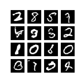
Stored notebook result
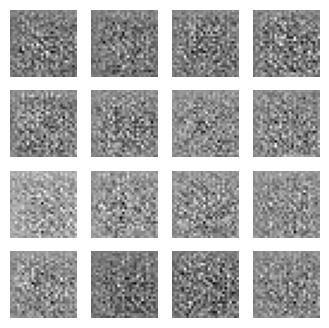
The stored output does not prove why this happened. Check the path, restored variables, and training state. A missing checkpoint can raise an error.
Run the full training loop
train(train_dataset, EPOCHS)
checkpoint.restore(tf.train.latest_checkpoint(checkpoint_dir))
The notebook defines a helper named display. This replaces the earlier IPython module name. Before running the GAN loop, use the fix below and replace both display.clear_output calls.
from IPython import display as ipy_display
# In train(), replace display.clear_output(wait=True) with:
ipy_display.clear_output(wait=True)
Verify a checkpoint before using it
checkpoint_path = "./pretrained_checkpoints/ckpt-2"
if not tf.io.gfile.exists(checkpoint_path + ".index"):
    raise FileNotFoundError(checkpoint_path)
# Build both models before checking restored model variables.
_ = generator(tf.zeros([1, 100]), training=False)
_ = discriminator(tf.zeros([1, 28, 28, 1]), training=False)
status = checkpoint.restore(checkpoint_path)
status.assert_existing_objects_matched()
predictions = generator(seed, training=False)
Added diagnostic code. Optimiser slot checks may require the slots to be created first.
Why keep the same noise seed for progress images?
Changing the seed changes the samples. A fixed seed makes changes across epochs easier to attribute to training.
Notebook source · 11 cells
Exact source and saved outputs. Python runs in Jupyter. Page controls use local teaching demos.
Cell 64 · Notebook text
#### Save checkpoints

This notebook also demonstrates how to save and restore models, which can be helpful in case a long running training task is interrupted.
Cell 65 · Python · checkpoint_dir = './training_checkpoints'
checkpoint_dir = './training_checkpoints'
checkpoint_prefix = os.path.join(checkpoint_dir, "ckpt")
checkpoint = tf.train.Checkpoint(generator_optimizer=generator_optimizer,
                                 discriminator_optimizer=discriminator_optimizer,
                                 generator=generator,
                                 discriminator=discriminator)
Cell 66 · Notebook text
#### Generate and save images
Cell 67 · Python · def generate_and_save_images(model, epoch, test_input):
def generate_and_save_images(model, epoch, test_input):
  # Notice `training` is set to False.
  # This is so all layers run in inference mode (batchnorm).
    predictions = model(test_input, training=False)

    fig = plt.figure(figsize=(4, 4))

    for i in range(predictions.shape[0]):
        plt.subplot(4, 4, i+1)
        plt.imshow(predictions[i, :, :, 0] * 127.5 + 127.5, cmap='gray')
        plt.axis('off')

    plt.savefig('image_at_epoch_{:04d}.png'.format(epoch))
    plt.show()
Cell 69 · Python · EPOCHS = 50 # In practice you need at least 20 epochs to generate nice
EPOCHS = 50 # In practice you need at least 20 epochs to generate nice digits.
noise_dim = 100
num_examples_to_generate = 16

# You will reuse this seed overtime (so it's easier)
# to visualize progress after each epoch
seed = tf.random.normal([num_examples_to_generate, noise_dim])
Cell 72 · Python · def train(dataset, epochs):
def train(dataset, epochs):
    for epoch in range(epochs):
        start = time.time()

        for image_batch in dataset:
            train_step(image_batch)

        # Produce images for each epoch
        display.clear_output(wait=True)
        generate_and_save_images(generator,
                                 epoch + 1,
                                 seed)

        # Save the model every 15 epochs
        if (epoch + 1) % 15 == 0:
            checkpoint.save(file_prefix = checkpoint_prefix)

        print ('Time for epoch {} is {} sec'.format(epoch + 1, time.time()-start))

    # Generate after the final epoch
    display.clear_output(wait=True)
    generate_and_save_images(generator,
                             epochs,
                             seed)
Cell 73 · Notebook text
### Train the model
Call the `train()` method defined above to train the generator and discriminator simultaneously. Note, training GANs can be tricky. It's important that the generator and discriminator do not overpower each other (e.g., that they train at a similar rate).

At the beginning of the training, the generated images look like random noise. As training progresses, the generated digits will look increasingly real. After about 50 epochs, they resemble MNIST digits.

To train your own model, run:

`train(train_dataset, EPOCHS)`

To restore the latest checkpoint with your own model, run:

`checkpoint.restore(tf.train.latest_checkpoint(checkpoint_dir))`

To save time, we will use the prepared checkpoints directly in the workshop.
Cell 74 · Python · import logging
# Optional: Disable Tensorflow verbose logging output
import logging
tf.get_logger().setLevel(logging.ERROR) # or any {DEBUG, INFO, WARNING, ERROR, CRITICAL}
Cell 75 · Python · checkpoint.restore("./pretrained_checkpoints/ckpt-2") #about 100 epoch
## Restore the pre-trained checkpoints
# checkpoint.restore("./pretrained_checkpoints/ckpt-1") #about 50 epochs
checkpoint.restore("./pretrained_checkpoints/ckpt-2") #about 100 epochs
Stored output
<tensorflow.python.checkpoint.checkpoint.CheckpointLoadStatus at 0x352bf8ca0>
Cell 76 · Python · predictions = generator(seed, training=False)
predictions = generator(seed, training=False)Cell 77 · Python · fig = plt.figure(figsize=(4, 4))
# Display the results
fig = plt.figure(figsize=(4, 4))

for i in range(predictions.shape[0]):
    plt.subplot(4, 4, i+1)
    plt.imshow(predictions[i, :, :, 0], cmap='gray')
    plt.axis('off')

plt.show()
Stored output
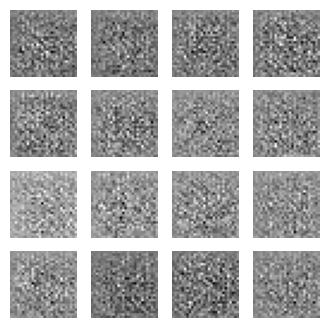
<Figure size 400x400 with 16 Axes>
What does the discriminator score?
Why this mattersCheck what the discriminator has learned to separate.
Try thisCompare real and fake logits. Use the images to interpret the scores.
Zero is the centre line. Left: favours fake. Right: favours real. The scale is fixed across both views.
All ten real scores were slightly negative. Fake scores sat near zero. That is not a working critic. It matches an unrestored $D$.
Should every generated image always receive a negative score?
The notebook expects positive real scores and negative fake scores for a discriminator that separates them.
This is not guaranteed. A strong generator can fool D. At ideal GAN equilibrium, both scores can approach zero. The saved noise-like images and weak scores call for further checks; scores alone do not prove a failed restore.
real_output = discriminator(x_test[:10], training=False)
fake_output = discriminator(fake_images, training=False)

print ("Scores for real images",real_output)
print ("Scores for fake images",fake_output)
Stored image pairs
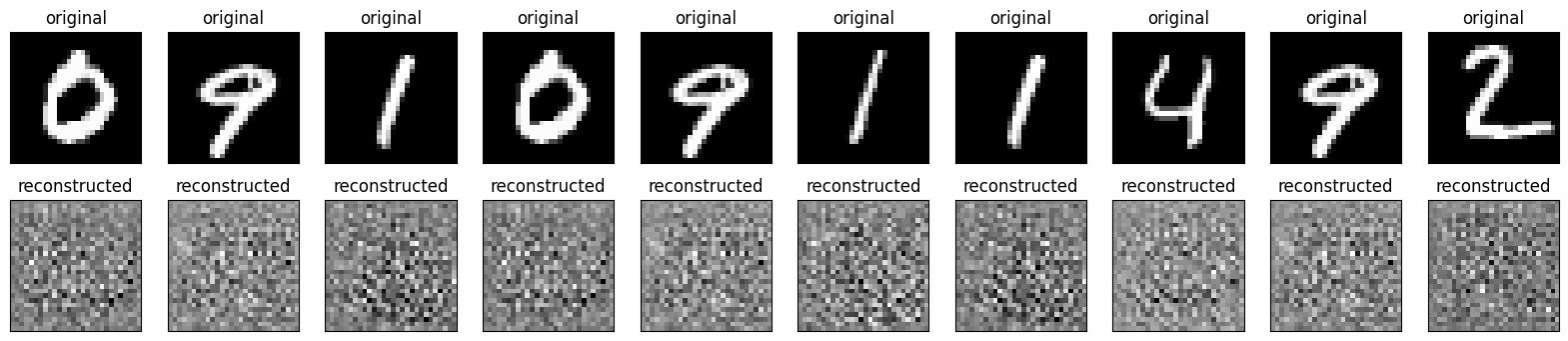
Notebook source · 5 cells
Exact source and saved outputs. Python runs in Jupyter. Page controls use local teaching demos.
Cell 78 · Notebook text
### Exercise 2: Check the Discriminator output for real and fake images

Run some real images (from a test set) and fake images (N random samples from the Generator) through the Discriminator and check their scores. If the Discriminator is well-trained, it should output positive values for real images, and negative values for fake images.
Cell 79 · Python · real_images = x_test[:10]
# Choose 10 real images for test set and generate 10 fake images from the Generator
real_images = x_test[:10]
noise = tf.random.normal([10, noise_dim])
fake_images = generator(noise, training=False)

display(real_images, fake_images.numpy())

# Run these real/fake images rough the Discriminator and check their scores.
# your code
Stored output
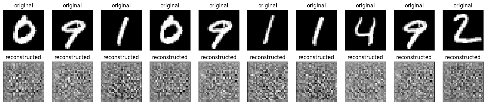
<Figure size 2000x400 with 20 Axes>
Cell 80 · Notebook text
The top row is the real images for the test set, and the bottom row is the fake images generated from the Generator.
Cell 81 · Notebook text
### Solution
Cell 82 · Python · real_output = discriminator(x_test[:10], training=False)
real_output = discriminator(x_test[:10], training=False)
fake_output = discriminator(fake_images, training=False)

print ("Scores for real images",real_output)
print ("Scores for fake images",fake_output)
Stored output
Scores for real images tf.Tensor(
[[-0.1127525 ]
 [-0.10259311]
 [-0.08745752]
 [-0.10899768]
 [-0.03588801]
 [-0.08322508]
 [-0.114327  ]
 [-0.07023349]
 [-0.03052524]
 [-0.08232151]], shape=(10, 1), dtype=float32)
Scores for fake images tf.Tensor(
[[ 6.1758328e-07]
 [ 3.8085919e-04]
 [-3.0598999e-03]
 [ 1.0995279e-03]
 [-1.1941220e-03]
 [-1.2221746e-04]
 [ 7.4083486e-04]
 [-2.5569103e-03]
 [-2.0648669e-03]
 [-1.3346837e-03]], shape=(10, 1), dtype=float32)
Is the generator copying?
Why this mattersLook for evidence that generated images copy the training data.
Try thisCompare a query with its three closest matches. Similar is not the same as identical.
The query is a held-out digit or its PCA reconstruction. Each search was computed across all 60,000 training images. This is not a GAN result.
How would you find the three closest training images?
Compare each training image with the generated image. Sort by pixel error and inspect the first three.
query = generator(tf.random.normal([1, 100]), training=False)[0]
# query: (28, 28, 1); x_train: (60000, 28, 28, 1)
mse = tf.reduce_mean(tf.square(x_train - query), axis=(1, 2, 3))
nearest = tf.argsort(mse)[:3]
for rank, idx in enumerate(nearest.numpy()):
    plt.subplot(1, 3, rank + 1)
    plt.imshow(x_train[idx, :, :, 0], cmap="gray")
    plt.axis("off")
plt.show()
Shape-corrected solution. The original uses tf.squeeze(x_train[i]). This can broadcast across mismatched axes and produce the wrong distance.
Original solution figures
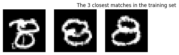
Notebook source · 4 cells
Exact source and saved outputs. Python runs in Jupyter. Page controls use local teaching demos.
Cell 83 · Notebook text
### Exercise 3: Check that generated images are not just copies of the training set

Is the Generator simply repeating images from its training set? Or has it learned how to create new images?

To check this, generate one random image from the Generator. Compute its similarity (e.g., sum of square pixel difference) to every image in the training set. Return the closest match (or 3 closest matches).
Cell 84 · Python · from sklearn.metrics import mean_squared_error, r2_score
from sklearn.metrics import mean_squared_error, r2_score
import heapq
from tqdm import tqdm

# your code
Cell 85 · Notebook text
### Solution
Cell 86 · Python · noise = tf.random.normal([1,100])
# Generate one random image from the Generator
noise = tf.random.normal([1,100])
gen = generator(noise, training=False)

plt.imshow(gen[0, :, :, 0] * 127.5 + 127.5, cmap='gray')
plt.title("Generated Image")
plt.axis('off')
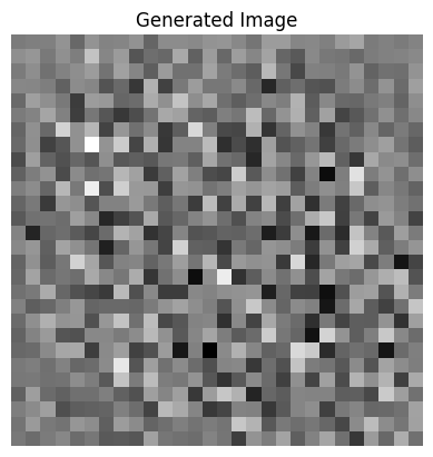
plt.show()

# Compute its similarity to every image in the training set.
# We use sum of square pixel difference as the similarity here.
similarity = []
for i in tqdm(range(len(x_train))):
    mse = tf.reduce_mean(tf.square(gen - tf.squeeze(x_train[i])))
    heapq.heappush(similarity, (mse,i))

# Find the three smallest value, i.e. the three most similar index
k = 3
results = []
for _ in range(k):
    results.append(heapq.heappop(similarity))

# Display the three closest matches found
for i, (_,idx) in enumerate(results):
    plt.subplot(1,3,i+1)
    plt.imshow(np.squeeze(x_train[idx]))
    plt.axis('off')

plt.title("The 3 closest matches in the training set")
plt.show()
Stored output
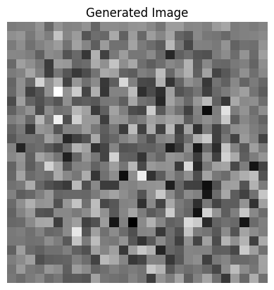
<Figure size 640x480 with 1 Axes>
100%|███████████████████████████████████| 60000/60000 [00:06<00:00, 9546.72it/s]
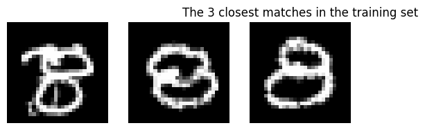
<Figure size 640x480 with 3 Axes>
Walk through latent space
Why this mattersTest whether nearby latent codes produce gradual, plausible changes.
Try thisMove from A to B. Watch the intermediate images, not just the endpoints.
Decode interpolated code
Interpolate decoded pixels
For an affine PCA decoder, these two paths are equal before clipping. A nonlinear generator can produce a different path.
What would continuity and completeness look like along the walk?
Continuity: small steps give gradual image changes.
Completeness: in the notebook’s intended test, all intermediate images look plausible. A good path does not prove that every latent point generates a real-looking digit.
Smooth output changes alone do not rule out memorisation.
# Select two random points in the Generator's input space.
noise = tf.random.normal([2, 100])

# Get 50 equally-spaced points from A to B
walking_latent = np.linspace(noise[0], noise[1], 50)
walking_latent_images = generator(walking_latent, training=False)

fig = plt.figure(figsize=(10, 5))

for i in range(walking_latent_images.shape[0]):
    plt.subplot(5, 10, i+1)
    plt.imshow(walking_latent_images[i, :, :, 0] * 127.5 + 127.5, cmap='gray')
    plt.axis('off')
Stored walk and baseline comparisons
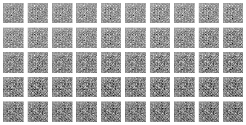


Notebook source · 4 cells
Exact source and saved outputs. Python runs in Jupyter. Page controls use local teaching demos.
Cell 87 · Notebook text
### Exercise 4: Do a linear walk through the latent space
In a well-trained generative model, the latent space should be **continuous** and **complete**. Continuous means that similar images are nearby in the latent space. Complete means that all points in the latent space correspond to real images.

A good way to check this is to do a linear walk through the latent space. Select two random points (A,B) in the Generator's input space. Get N equally-spaced points from A to B (e.g., from `numpy.linspace`) and generate an image for each of those input points.

If the GAN is well-trained, the images should show a smooth transition from A to B (indicating that the latent space is continuous) and every step between those points should look like a realistic image (indicating that the latent space is complete).
Cell 88 · Python · Exercise space
# your codeCell 89 · Notebook text
### Solution
Cell 90 · Python · noise = tf.random.normal([2, 100])
# Select two random points in the Generator's input space.
noise = tf.random.normal([2, 100])

# Get 50 equally-spaced points from A to B
walking_latent = np.linspace(noise[0], noise[1], 50)
walking_latent_images = generator(walking_latent, training=False)

fig = plt.figure(figsize=(10, 5))

for i in range(walking_latent_images.shape[0]):
    plt.subplot(5, 10, i+1)
    plt.imshow(walking_latent_images[i, :, :, 0] * 127.5 + 127.5, cmap='gray')
    plt.axis('off')
Stored output
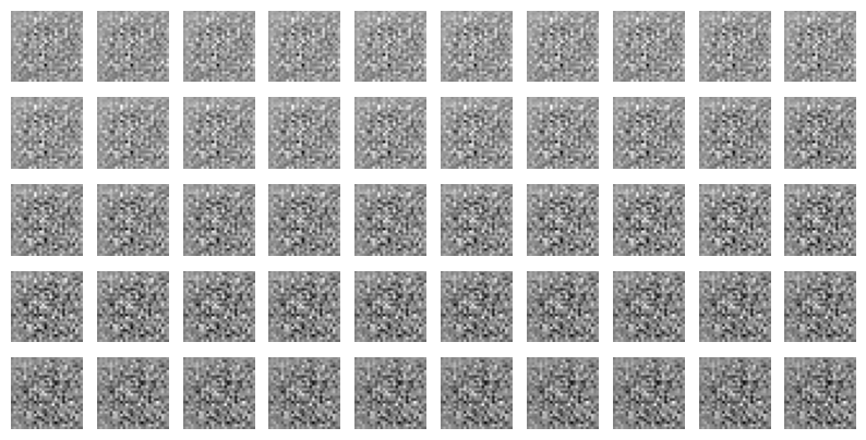
<Figure size 1000x500 with 50 Axes>
How many different images?
Why this mattersDetect a generator that repeats a small set of images.
Try thisFirst count birthday pairs. Then replace birthdays with possible generated images.
23 people. A surprisingly likely match.
A match can occur between any two people. Each new person adds several new pairs.
One dot = one person. One line = one chance to match. Lines do not show actual shared birthdays.
We often think about one person’s birthday. The test compares every pair. With 23 people, there are 23 × 22 / 2 = 253 pairs.
Assume independent birthdays, 365 equally likely days, and no leap day. The bars use the exact probability under these assumptions.
Why count “no match” first?
Person 1 can have any birthday. Person 2 must avoid 1 day. Person 3 must avoid 2 days. Continue this pattern.
This product is the chance that all birthdays differ. Subtract it from 1 to get the chance of at least one match.
$$P(\text{match})=1-\prod_{i=0}^{N-1}\left(1-\frac{i}{365}\right)$$We do not treat the pair events as independent. Multiplying the “new birthday” chances gives the exact result.
People become samples. Birthdays become outputs.
Draw birthdays from 365 possible days.
Draw from S possible distinct outputs.
A collision is a repeated output. If repeats appear in small batches, the generator may have limited variety.
S is the support size: the number of possible outputs in this simplified model. Real GAN outputs need a clear near-duplicate rule.
Keep N fixed and reduce S. Watch the repeat probability rise. This estimates a batch-level chance, not a count from one grid.
Synthetic sample. Larger red dots mark repeated categories.
Why N²? A batch has N(N − 1) / 2 pairs. That count grows roughly as N². Under uniform sampling, a 50% repeat chance occurs when N is on the order of √S.
If half of the N = 50 batches contain a duplicate, how large is the support?
The notebook’s rule of thumb is N² = 2,500 images.
The uniform-support approximation gives S ≈ N(N − 1) / (2 ln 2), or about 1,767. The difference is the constant in the approximation.
Real GANs are not uniform. Near-duplicate thresholds also affect the estimate. Treat this as a diversity diagnostic.
N = 50

noise = tf.random.normal([N, noise_dim])
generated_images = generator(noise, training=False)

fig = plt.figure(figsize=(10, 5))

for i in range(generated_images.shape[0]):
    plt.subplot(5, 10, i+1)
    plt.imshow(generated_images[i, :, :, 0] * 127.5 + 127.5, cmap='gray')
    plt.axis('off')
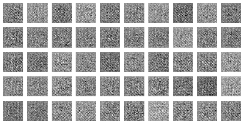
Collision formula and notebook grid
The calculator uses this formula. The coloured dots are a synthetic example of repeated categories.
Notebook source · 2 cells
Exact source and saved outputs. Python runs in Jupyter. Page controls use local teaching demos.
Cell 91 · Notebook text
### Exercise 5: Implement [the birthday paradox test](https://arxiv.org/abs/1706.08224)

Ideally, a generative model should be able to produce a wide variety of images. However, in practice GANs usually show some amount of "mode collapse" -- the Generator can only produce a limited number of images. In severe cases of mode collapse, a Generator will only learn to produce a single image.

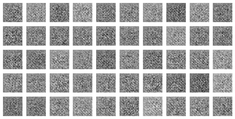
Less-severe cases of mode collapse are hard to detect, but one way to check for this is the [the birthday paradox test](https://arxiv.org/abs/1706.08224). Choose a value of N and generate N random images. See if you can spot any duplicate images in the set of N. The value of N at which you start seeing duplicates gives you an approximation of the number of images the GAN can produce. If you have a 50% chance of duplicates in a set of N, that suggests that the Generator produces approximately N^2 unique different images.
Cell 92 · Python · N = 50
N = 50

noise = tf.random.normal([N, noise_dim])
generated_images = generator(noise, training=False)

fig = plt.figure(figsize=(10, 5))

for i in range(generated_images.shape[0]):
    plt.subplot(5, 10, i+1)
    plt.imshow(generated_images[i, :, :, 0] * 127.5 + 127.5, cmap='gray')
    plt.axis('off')
Stored output
<Figure size 1000x500 with 50 Axes>
Quality can rise as diversity falls
Why this mattersSeparate image recognisability from variety across a batch.
Try thisChange classifier confidence and class coverage. Watch when the score rises or falls.
The notebook’s training story: quality rises, variety falls
Clear predictions. A varied batch.
A classifier gives each image class probabilities. The score compares each image’s prediction with the batch average.
Each image · p(y | x)
A narrow prediction means “I recognise this”.
Batch average · p(y)
Average the probabilities across all six images.
Variety across the batch
Uncertainty per image
Entropy measures spread. We want a broad batch average and focused individual predictions.
What can a high score miss?
The example uses two different handwritten images per class.
A classifier can stay confident even when a generator repeats images. This score does not test whether images are copied from the training set.
Use the birthday test and nearest-neighbour checks alongside it. Classifier confidence is a useful signal, not proof of visual quality.
Connect the picture to the formula
Purpose: reward confident predictions for individual images and broad class coverage across the batch.
$$\mathrm{IS}=\exp\left(\frac1N\sum_{i=1}^{N}D_{\mathrm{KL}}\bigl(p(y\mid x_i)\,\|\,p(y)\bigr)\right)$$xᵢ: one generated image. y: a class. p(y | xᵢ): the classifier’s probabilities for that image. p(y): their average over the batch.
KL measures how much each prediction differs from the batch average. The exponential turns the average KL into the reported score.
$$\log\mathrm{IS}=H(p(y))-\frac1N\sum_i H(p(y\mid x_i))$$Entropy H measures uncertainty. We want high class variety in the batch and low uncertainty for each image. Values here use natural logarithms, measured in nats.
If every image has the same probability vector, the two terms cancel. The score is 1.
Teaching example: real MNIST images with chosen probability vectors. No classifier runs here. The original Inception Score uses an Inception classifier; a digit classifier gives an analogous score for MNIST.
Sources: Salimans et al. · Barratt & Sharma on limitations.
i. How could the developer measure quality?
Notebook answer: Inception Score.
It uses a classifier’s confidence and the spread of predicted classes. It also reflects some diversity. It can miss repetition within a class. For MNIST, a suitable digit classifier is more relevant than an ImageNet classifier.
ii. How could the developer measure diversity?
Notebook answer: the birthday paradox test.
Generate repeated batches and inspect near-duplicates. More collisions can indicate a smaller effective support.
iii. Why could diversity drop later in training?
Notebook answer: the discriminator overfits.
This is a possible cause, not a diagnosis from images alone. The generator may focus on a few outputs that fool D. This is mode collapse.
Notebook source · 2 cells
Exact source and saved outputs. Python runs in Jupyter. Page controls use local teaching demos.
Cell 93 · Notebook text
### Exercise 6

A Generative Adversarial Network is being trained. The developer observes that initially the Generator is creating images that look like patterned snow.  After some training, it is starting to generate blurry images that start to look like the training data. Later the quality of the generated  images increases but the diversity drops.

i) How might the developer measure quality?

A: Inception score

ii) How might the developer measure diversity?

A: Birthday paradox

iii) Why might diversity drop during the later part of training?

A: Discriminator overfits
Cell 94 · Python · Exercise space
# Empty exercise cell in the source notebook.Choose the model. Choose the check.
Why this mattersChoose an evaluation check that answers your actual question.
Try thisMatch each model to its training signal. Then choose a check for repeated images.
| Autoencoder | VAE | GAN (DCGAN) | |
|---|---|---|---|
| Maps | $x\to z\to\hat{x}$ | $x\to(\mu,\sigma)\to z\to\hat{x}$ | $z\to G(z)$; $D$ scores images |
| Latent | Unconstrained code | $q_\phi(z\mid x)$ near $\mathcal{N}(0,I)$ | Prior $z\sim\mathcal{N}(0,I)$ only |
| Loss | $\ell(x,\hat{x})$ | reconstruction $+$ KL | $\min_G\max_D V(D,G)$ |
| Sampling | No simple $p(z)$ | Draw $z\sim p(z)$, decode | Draw $z\sim p(z)$, generate |
| Typical look | Slightly blurry copy | Blurrier, more regular | Often sharp; training can be unstable |
| Failure | Lost detail; overfitting | Unused latent codes; excessive blur | Mode collapse; $D$ overfitting |
| Workshop check | Recon grid + t-SNE; vary $k$ | ELBO terms; 2-D latent grid | Scores, neighbours, walk, birthday |
A generator repeats one convincing digit. Which checks would reveal the problem?
Use the birthday test and inspect class coverage. Nearest neighbours test possible training copies. A latent walk tests changes along selected paths. Realistic appearance alone does not measure diversity.
Optional tools and references
- Keras autoencoder tutorial
- TensorFlow autoencoders
- TensorFlow convolutional VAE
- TensorFlow DCGAN
- scikit-learn t-SNE reference
- GAN Lab
- ConvNetJS autoencoder
- VAE Explainer
- Kingma & Welling: Auto-Encoding Variational Bayes
- Goodfellow et al.: Generative Adversarial Nets
- Radford et al.: DCGAN
- Arora & Zhang: birthday test
- Salimans et al.: Inception Score
- Keenan Crane, Autoencoder Diagrams (2025), CC0.