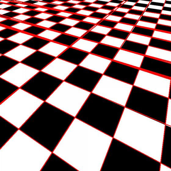
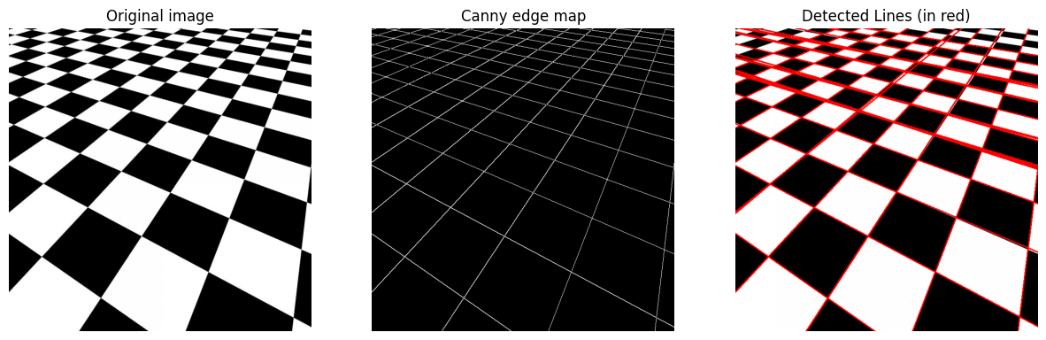
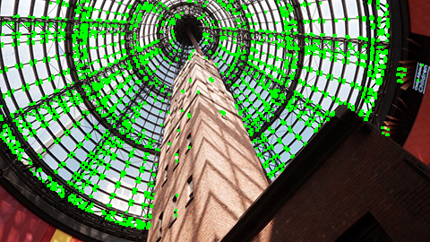
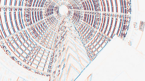
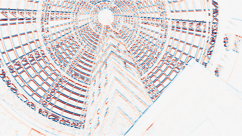
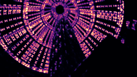
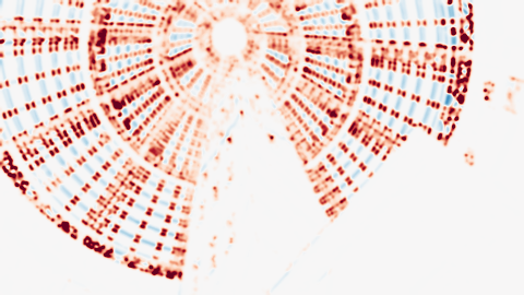
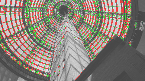
Canny is one way to get an edge map. A binary boundary mask can also feed Hough. For noisy input, Gaussian smoothing can be applied first; this notebook passes the grayscale image directly.
Aperture size is the width and height of the Sobel kernel, in pixels.
Choose the footprint
Same noisy step edge. Orange box = pixels used for one derivative.
Horizontal-change kernel
Negative weights on the left; positive on the right. Equal intensities cancel.
Derivative image · same colour scale
Red = increasing brightness. Blue = decreasing brightness.
One horizontal slice through the centre
Profiles divide by each kernel’s ramp gain, so a unit ramp gives 1 for every size. Raw Sobel values have different scales: retune Canny thresholds when changing aperture.
Work one raw 3 × 3 Sobel calculation
A clean vertical edge: every row changes from 10 to 110.
The perpendicular form handles both. Use 0° ≤ θ < 180° and a signed ρ; a negative ρ points opposite the chosen normal.
02 / Find lines
Find lines · 2 of 4
Pixels vote for a line
Keep P = (4, 3). Follow its votes, then add pixels to find the line they share.
1 / 4 · One vote
P votes for a diagonal line
At θ = 45°, P gives ρ ≈ 4.95. Mark this pair in the vote plot.
Image · where are the pixels?
Votes · which lines could contain them?
Explore freely: drag pixels, try vertical lines or add outliers
Nearby votes → one peak group → refine the line. Yellow lines and rings use the same fitted parameters.
Image points ↔ line parameters
Image space $(x, y)$origin top-left, y down (OpenCV)
Enter: select a point · arrows: move it. Or drag in the image.
Parameter space $(\theta, \rho)$θ: 0°→180°, ρ: −D→+D
One coloured curve per pixel. Yellow rings use the same θ and ρ as the fitted lines.
1edge pixels
1pixels supporting line
–line θ · refined
–line ρ (px)
One pixel → one curve. Add another pixel to find a shared crossing.
02 / Find lines
Find lines · 3 of 4
Keep the strongest votes
Each bright cell counts pixels that support a line. Keep cells with at least T votes.
Try it Raise T. Watch the line count fall while the accumulator stays the same.
Vote threshold
40
Edge pixels + detected lines128 × 128
White = Canny edge pixel (each casts 180 votes). Red = every accumulator cell with votes ≥ T, drawn back as a line.
Accumulator $A[\rho,\theta]$brightness = votes
–edge pixels
–max votes in a cell
–lines ≥ T
Inspect the full accumulator
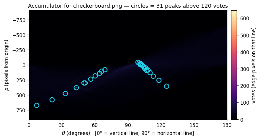
The full $1813\times180$ accumulator of the checkerboard edge map ($\rho$ resolution 1 px, $\theta$ resolution 1°). Bright cells are lines with many votes; cyan circles are the 31 cells that cv2.HoughLines(..., threshold=120) returns. The two curved families of peaks are the two sets of parallel grid lines, bent by perspective: each family converges to a vanishing point, so its $\theta$ drifts smoothly with $\rho$.
Why do peaks look like short streaks, not dots? A thick or slightly curved edge spreads votes over neighbouring $\rho$ and $\theta$ bins. That is why one physical line can produce two or three detections a few pixels apart.
Bin size trade-off. Coarser bins (say 3°) merge nearby votes and make peaks taller but blur distinct parallel lines together. Finer bins separate lines but scatter the votes of an imperfect line.
Reading this result
Reading θ. Peaks near $\theta\approx100^\circ$ are the nearly-horizontal lines of the board; peaks near $\theta\approx 10^\circ$–$70^\circ$ are the receding lines. Nothing sits near $\theta = 150^\circ$ because no edge in this image has that orientation.
02 / Find lines
Find lines · 4 of 4
Try the worksheet image
Use the full-resolution results to choose a threshold.
Try it Compare T = 40, 120 and 300.
Exercise 1 · full-resolution output
120
Number of returned lines vs threshold (log scale)
31lines returned
14 093edge pixels
Notebook answer & code
Fewer / more lines (but with lower thresholds, the lines may be worse, since they will be accepted with fewer "votes"). The code is only a reference solution; the aim is to understand the effect of the parameters, so different parameters are accepted.
Lower T → more lines, lower quality. At T = 40 the checkerboard returns 1338 "lines"; most are near-duplicates of real grid lines plus diagonals through the square corners that happen to collect 40 votes.
Higher T → fewer, longer lines. At T = 120 you get 31 lines (the grid); at T = 300 only 6 survive; at T = 400 just 2. Short receding lines at the top of the board lose out first because they contain fewer edge pixels.
The threshold is in units of edge pixels, so it must be tuned per image and per resolution. A 640-px-long edge can score ~640 votes; a 100-px edge can never pass T = 120 however perfect it is.
Canny first. Hough needs a sparse binary input. Feeding it a grayscale image (every pixel votes) floods the accumulator.
Keep the same shift throughout. Each step is another way to write its local cost.
Local shift cost · same toy window
Centre = no shift. Move the dot; brighter means more change.
Pixel 1 · weight 1
Pixel 2 · weight 1
This toy window has gradients $(2,1)$ and $(0,1)$, with weights 1. The plot shows the local quadratic model, not a claim that real images stay linear for large shifts.
Dot = this window (trail = recent positions). Shading uses the same rule as the verdict: green where $R>0.02\,R_{\max}$ (corner), red where $\lambda_1$ is large but $R$ is not (edge), grey near the origin (flat). Both axes run to the 98th percentile of $\lambda_1$ in this image; the dashed line is $\lambda_1=\lambda_2$.
Gradient vectors $(I_x, I_y)$ of the window pixels
$I_x\rightarrow$$I_y\downarrow$
Each dot is one gradient $(I_x,I_y)$. The ellipse shows the second moment about zero: radii $\sqrt{\lambda_1}$ and $\sqrt{\lambda_2}$. It is not a mean-centred covariance ellipse. In shift space, equal-cost radii vary inversely as $1/\sqrt{\lambda_i}$.
Numbers for this window
This explorer normalises window weights to sum to 1. The response has the same shape as the weighted-sum definition, at a different scale.
Scroll horizontally. Notice that $\lambda_1$ is bright on every edge, but $\lambda_2$ is bright only where two edge directions meet — that is the whole trick. The window here is a Gaussian with $\sigma=1.5$; OpenCV's cornerHarris(blockSize=2) uses a 2×2 box instead.
What happens when the image gets larger?
Same corner, same 9-px window, image zoomed 3×
The response depends on the window size relative to the structure. The eigenvalues of $\mathbf M$ do not change if you rotate the image (rotation invariance), but they do change if you scale it. Fix: search over scale as well — Primer 3.
What Harris gives you, and what it does not
Property
Harris
Translation / rotation
invariant (eigenvalues of $\mathbf M$)
Brightness shift $I+b$
invariant (gradients unchanged)
Contrast scale $aI$
$R$ scales by $a^4$ → threshold must be relative ($\alpha R_{\max}$)
Image scale
not invariant
Descriptor for matching
none — Harris only says where
04 / Describe features
Describe features · 1 of 4
Search across image scales
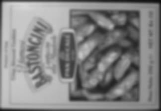
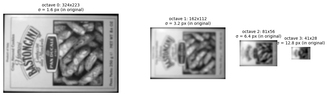
Blur twice, then subtract. Larger blur reveals larger structures.
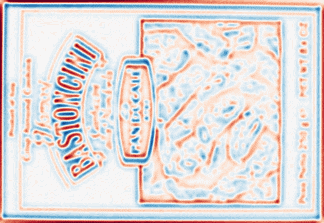
Difference of Gaussians ≈ scale-normalised Laplacian
$$D(x,y,\sigma)=L(x,y,k\sigma)-L(x,y,\sigma)\approx(k-1)\,\sigma^2\nabla^2 G * I$$
Octaves
Extremum in $x$, $y$ and $\sigma$
04 / Describe features
Describe features · 2 of 4
Keep stable keypoints
Compare each candidate with 26 neighbours across space and scale.
Strong contrast ✓Local peak or valley ✓Edge-like ridge ×
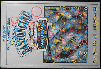
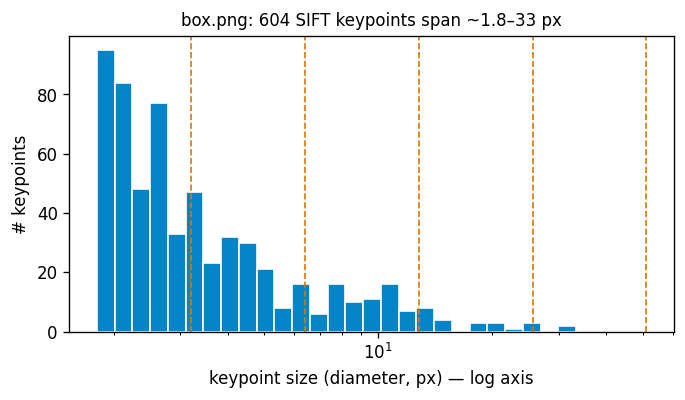
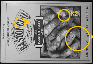
The 604 keypoints OpenCV finds in box.png , circle radius = keypoint size/2.
Sizes span more than a factor of 30, roughly one cluster per octave (dashed lines are one octave apart). No single window size — this is what Harris could not do.
$$\text{accept}\iff \frac{d_1}{d_2}<\tau\qquad(\tau=0.7\text{ in the notebook})$$
Numbers
$d_1=120,\ d_2=310$ratio 0.39 → keep (distinctive)$d_1=205,\ d_2=225$ratio 0.91 → reject (ambiguous)$d_1=40,\ d_2=46$ratio 0.87 → reject — small distance, still ambiguous!
05 / Match features
Match features · 2 of 2
Filter real matches
A smaller ratio threshold keeps fewer, more distinctive pairs.
Try it Move τ from 0.7 toward 0.9. Watch the wrong matches appear.
Keep distinctive matches
0.70
accepted & correct accepted but wrong rejected by the ratio test (faint)
Histogram of $d_1/d_2$ — the Lowe plot for this image pair
Green: nearest neighbour is correct (reprojection error < 5 px under the reference homography).
–pass the test ("good")
–of which correct
–precision
–recall (of 89 correct NN)
Reading this result
How reference labels are obtained
Ground truth here is the homography fitted with 10 000 RANSAC iterations on the 0.7-ratio matches (72 inliers). Only 89 of the 604 nearest neighbours are correct at all: the other 515 query points lie on background/side faces that are not visible, or are simply wrong.
$t$: distance tolerance · retain the largest consensus, then refit
06 / Reject outliers
Reject outliers · 2 of 3
Build one iteration, one action at a time
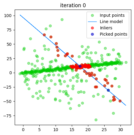
Sample → fit → count → keep. Then try another sample.
Try it Press the blue button four times to complete one iteration.
Fit a line among outliers
Noise, tolerance & stopping ruleoutliers 40% t 3 stop ratio 0.6
1 Sample2 Fit3 Count4 Keep
data the 2 sampled points candidate line its inliers best model so far least-squares refit on inliers least squares on everything
0iteration
–inlier ratio (this sample)
0.00best ratio so far
–best m
–best c
–true m (hidden from RANSAC)
Best inlier ratio vs iteration
Iteration log
press "step" …
Press Sample to choose two points.
Compare with the recorded notebook run
0
Iteration 7 → 65.4 % inliers > 0.6 → "The model is found!" Iteration 1 had an inlier ratio of 0.8 % — a sample of two outliers. The best model only ever improves (18 % → 19.2 % → 22.8 % → 58 % → 65.4 %).
Notebook answer & code
for it in range(ransac_iterations):
    # (1) randomly sample n = 2 points
    all_indices = np.arange(x_noise.shape[0]); np.random.shuffle(all_indices)
    sample_points = data[all_indices[:2], :]; test_points = data[all_indices[2:], :]

    # (2) fit a line model to the sampled points
    m, c = find_line_model(sample_points)

    # (3) count the inliers: distance to the line < ransac_threshold
    num = 0; x_list, y_list = [], []
    for x0, y0 in test_points:
        if find_dist_to_line(m, c, x0, y0) < ransac_threshold:
            x_list.append(x0); y_list.append(y0); num += 1

    if num / float(n_samples) > ratio:            # keep the best model
        ratio, model_m, model_c = num / float(n_samples), m, c
    if num > n_samples * ransac_ratio:             # good enough → stop
        print('The model is found !'); break
Compare least squares on all points with the consensus fit. Outliers can distort the all-point fit.
Refit on the consensus to reduce sample noise. Outliers inside the tolerance can bias the refit, so improvement is not guaranteed. The live demo uses orthogonal least squares and counts all points; the notebook uses y-on-x regression and excludes the sampled pair.
Expected iterations: $w=0.6,\ s=2$ → $w^2=0.36$ → $N=\ln(0.01)/\ln(0.64)\approx 11$ for 99 % confidence, consistent with finding it at iteration 7 here.
Threshold $t$ should match the noise: $t = 3\sigma$ keeps 99.7 % of true inliers. Too small and $w$ collapses; too large and outliers get counted.
06 / Reject outliers
Reject outliers · 3 of 3
How many attempts are enough?
The clean-sample probability determines the iteration budget.
$H$: 3 × 3 matrix, up to scale · four pairs in general position
Source plane → warped image
Move corner:← ↑ ↓ →
Synthetic checkerboard. Drag a pin, or select a pin below and use arrow keys. Dashed/grey lines show the mapped grid.
$\mathbf H$ solved from the 4 pin correspondences (normalised so $h_{33}=1$)
8degrees of freedom
0$|h_{31}|+|h_{32}|$ (perspective)
projectivemap type
Try: move only one pin. All 8 numbers change — a homography is a global model; that is exactly why a single wrong match can wreck a least-squares fit, and why we need RANSAC.
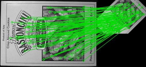
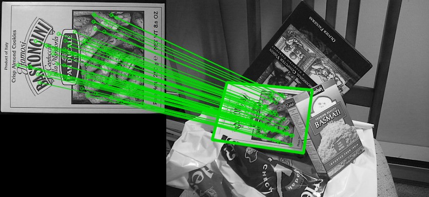
Green lines: the 72 RANSAC inliers. The green quadrilateral is the border of box.png pushed through $\mathbf H$ into the scene (cv2.perspectiveTransform) — the object is found.
$\mathbf H$ returned by cv2.findHomography(ptsA, ptsB, cv2.RANSAC, 5)
Read it: the box appears at ≈ 0.42× scale, slightly rotated (off-diagonal −0.16), translated to (119, 161), with a small perspective term in the last row.
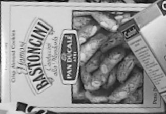
warpPerspective(scene, H, WARP_INVERSE_MAP): the scene pulled back into the template's frame. A good $\mathbf H$ makes the scene box look like the template.
08 / Find a landmark
Find a landmark · 1 of 1
Connect the whole pipeline
Choose an image pair, filter the matches, then fit the plane.
Try it Try Old Arts: keep τ = 0.8, compare 10 attempts with 200.
Match → fit → verify
0.60
100
Inlier tolerance
5
RANSAC inliers passed ratio test, rejected by RANSAC failed ratio test close-up border projected by the estimated $\mathbf H$
–keypoints (close-up / scene)
–pass ratio test
–reference-consistent matches
–inlier fraction w
–inliers found this run
–chance of a clean sample
–reference recovery / 50 runs
Probability that N draws contain ≥ 1 all-inlier sample, for this pair's w
Curve: clean-sample probability, with distinct points per draw. Green dots: measured reference recovery.
Run log
How the comparison is measured
A recovered model must map at least 75% of reference-consistent matches within 5 px (minimum 4). The reference is an estimated homography, not hand-labelled ground truth. The curve measures a clean draw; this does not guarantee recovery.
Notebook answer & code
Both of these are a bit more difficult than the box scene, so they may require a different ratio (which changes the number of good matches and percentage of false matches). They may also require a higher number of RANSAC iterations to find a correct solution. Different parameters are accepted.
Pair
keypoints
τ used
pass ratio test
truly correct
RANSAC inliers (solution run)
maxIters used
box → scene
604 / 969
0.7
74
72
72
10
Flinders Street
1910 / 4123
0.6
9
6
6
500
Old Arts tower
569 / 3555
0.8
39
15
17
200
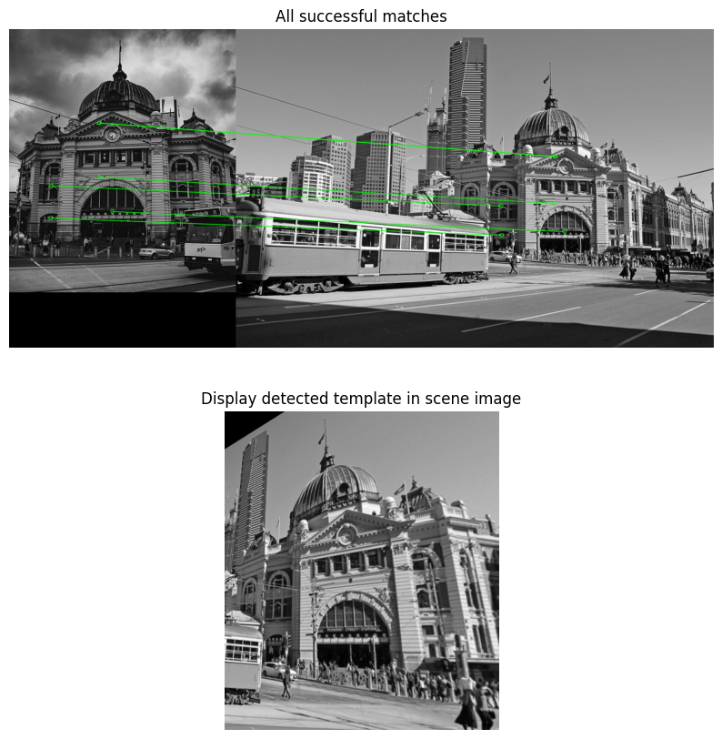
Ratio τ trades quantity for purity. Flinders: at τ = 0.7 there are 29 "good" matches but only 9 are correct (w ≈ 0.31); at τ = 0.6 there are 9 with 6 correct (w ≈ 0.67). Lowering τ makes RANSAC's job easier but leaves very few points to fit $\mathbf H$ — there is a floor at 4.
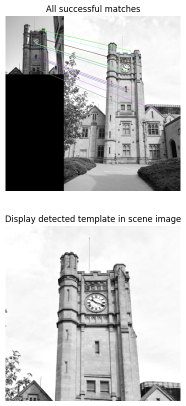
Raising τ when there are too few matches. The tower at τ = 0.7 keeps only 9 matches (6 correct); the solution relaxes to 0.8 to get 39 (15 correct). Fewer than ~8 inliers makes $\mathbf H$ unstable even when RANSAC succeeds.
More attempts increase the chance of a clean sample. They do not guarantee an accurate homography: repeated or poorly spread features can still produce degenerate geometry.
OpenCV's RANSAC is randomised, so re-running the same cell gives different inlier counts (15–17 for the tower). Use the "run 50 trials" button above to see the spread.
Official solution: Flinders, τ = 0.6, maxIters = 500 → 6 inliers; bottom: scene warped into the close-up frame.
Official solution: Old Arts, τ = 0.8, maxIters = 200 → 17 inliers.
09 / Fit a circle
Fit a circle · 1 of 2
A circle needs three points
Find the centre (a, b) and radius r from three non-collinear points.
$$(x-a)^2+(y-b)^2=r^2\qquad s=3$$
The input (from the worksheet).
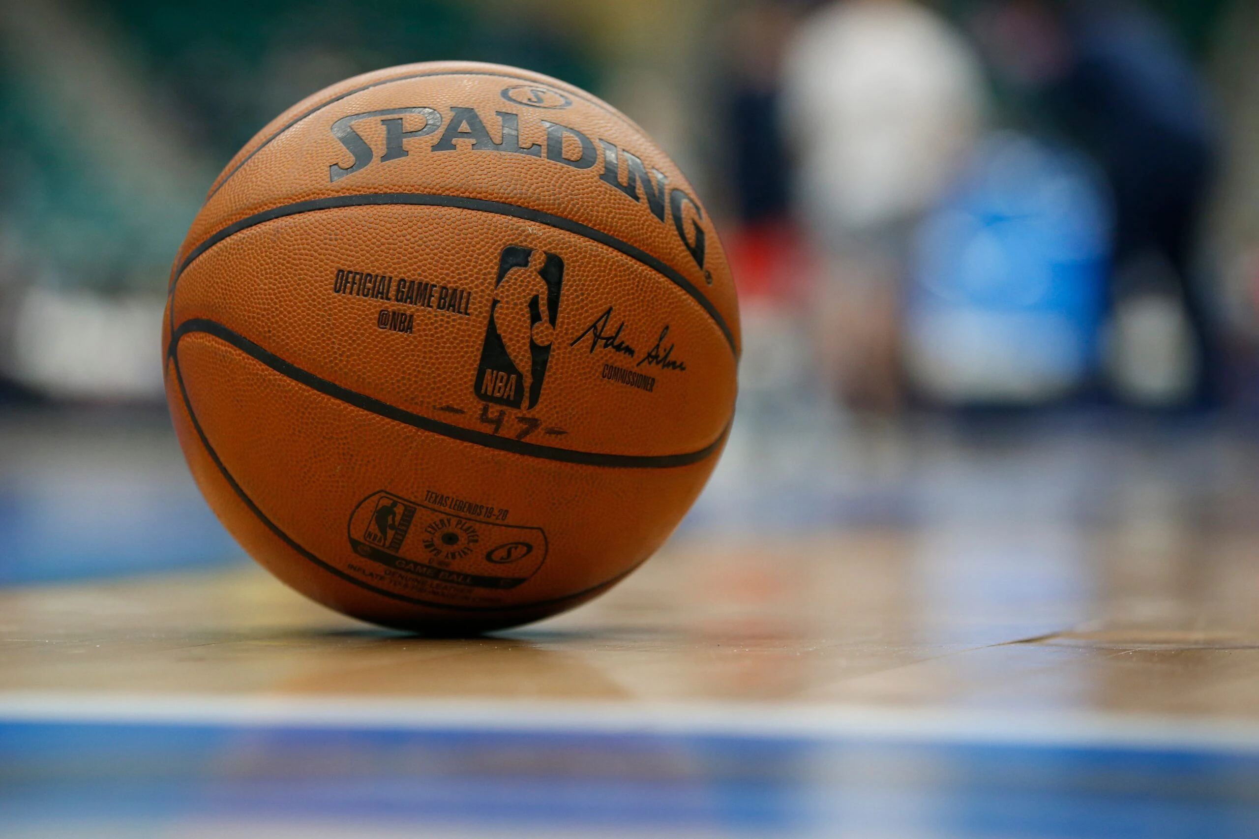
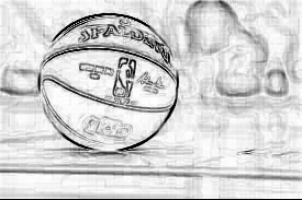
Its edge map: the ball's outline is a small minority of the edge pixels — the rest are logos, seams, floor lines, background.
Why 3 points?
$$(x-a)^2+(y-b)^2=r^2$$
Three unknowns $(a,b,r)$, so three non-collinear points pin down exactly one circle (the circumcircle). $s=3$.
SIFT:Lowe 2004, IJCV (σ = 1.6, $k=2^{1/3}$, contrast 0.03, edge ratio 10, 36 bins, 0.2 clip, ratio 0.8 — Fig. 11 motivates the ratio histogram; the workbook uses workshop-image data); Weitz's interactive SIFT lets you step every stage on your own image; CMU 16-385 Lecture 6.