Vision Transformers & Grad-CAM:
Seeing What Neural Networks See
An interactive workbook for visual explainability. Compare the global self-attention routing of Vision Transformers (ViT) with the gradient-weighted spatial feature attribution of Convolutional Neural Networks (Grad-CAM).
fruits.jpg (Primer 5 & Q5).
ViT 101: From Pixels to Tokens
Before classifying images with ViT, see how a 2D image is sliced into a 1D sequence of "words" that a standard Transformer encoder can digest.
Transformers expect a 1D sequence of token embeddings $\mathbf{z} \in \mathbb{R}^{N \times D}$. To process a 2D image $\mathbf{x} \in \mathbb{R}^{H \times W \times C}$:
1. Cut into $N = \frac{HW}{P^2}$ non-overlapping patches of size $P \times P = 16 \times 16$. For $224 \times 224$, $N = \frac{224 \times 224}{16 \times 16} = 14 \times 14 = \mathbf{196}$ patches.
2. Flatten each patch into $\mathbf{x}_p \in \mathbb{R}^{P^2 C}$. In the general formulation of Dosovitskiy et al., linear projection matrix $\mathbf{E} \in \mathbb{R}^{(P^2 C) \times D}$ maps each patch to latent dimension $D$: $$\mathbf{e}_i = \mathbf{x}_p^i \mathbf{E} \in \mathbb{R}^D$$ (Note: In ViT-Base, $P=16, C=3 \implies P^2 C = 768$ and $D=768$, so the dimensions happen to match ($768 \times 768$). In ViT-Large with $D=1024$, $\mathbf{E} \in \mathbb{R}^{768 \times 1024}$. Mentioning this avoids confusion when comparing architectures.)
3. Prepend a learnable [CLS] token $\mathbf{x}_{\text{class}}$ ($\to 197$ tokens) and add learnable 1D position embeddings $\mathbf{E}_{\text{pos}}$ because self-attention is permutation-invariant!
Classifying Images with ViT
Replace the sample image with your own image examples. How accurate are the classification results?
In ViT, all $197$ tokens pass through $L = 12$ Transformer encoder blocks. At the output of block 12, token 0 (the [CLS] token) has collected information from every patch in the image via self-attention. It passes through an MLP classification head to produce 1000 ImageNet logits:

For standard ImageNet categories (e.g. tabby cat, dingo, Maltese dog), the pre-trained ViT achieves extremely high top-1 accuracy (>90% confidence), demonstrating that patch-based tokenization with self-attention matches or exceeds deep CNNs.
Worth adding in class:
- Pretraining matters: ViT has less inductive bias than a CNN (no hardcoded spatial locality or translation equivariance). ViT only outperforms CNNs when pretrained on massive datasets (ImageNet-21k with 14M images or JFT-300M).
- Multi-object ambiguity: On images like
fruits.jpgcontaining both apples and bananas, the single[CLS]token is forced to summarize the entire scene into one label, causing prediction confidence to fragment across multiple classes. This motivates explainability techniques like Grad-CAM and Attention Rollout.
Self-Attention 101: Queries, Keys, Values & Heads
How do tokens communicate? Every token simultaneously asks: "Which other tokens in the image are relevant to me?"
For input token representations $\mathbf{X} \in \mathbb{R}^{N \times D}$, each head projects tokens into Queries $\mathbf{Q} = \mathbf{X}\mathbf{W}_Q$, Keys $\mathbf{K} = \mathbf{X}\mathbf{W}_K$, and Values $\mathbf{V} = \mathbf{X}\mathbf{W}_V$:
$$\mathbf{A} = \mathrm{softmax}\left(\frac{\mathbf{Q}\mathbf{K}^{\mathsf{T}}}{\sqrt{d_k}}\right), \qquad \mathrm{Attention}(\mathbf{Q}, \mathbf{K}, \mathbf{V}) = \mathbf{A}\mathbf{V}$$• $\mathbf{A}_{i,j}$ represents how much token $i$ attends to token $j$. Each row sums to $1.0$.
• Dividing by $\sqrt{d_k}$ (here $\sqrt{64} = 8$) prevents dot products from growing large in high dimensions, which would push softmax into near-zero gradient regions.
To see how spatial attention emerges from linear algebra, consider $N = 3$ tokens with $d_k = 3$ semantic dimensions:
• Dimension 1: Face / Eye feature | Dimension 2: Fur texture | Dimension 3: Background context
| [CLS] | 2.0 | 1.0 | 0.0 |
| Eye | 3.0 | 1.0 | -0.5 |
| Bg | 0.0 | 0.2 | 2.0 |
| [CLS] | Eye | Bg | |
| d₁ | 1.0 | 2.5 | 0.0 |
| d₂ | 1.0 | 1.0 | 0.5 |
| d₃ | 0.0 | -0.5 | 2.0 |
| [CLS] | Eye | Bg | |
| [CLS] | 3.00 | 6.00 | 0.50 |
| Eye | 4.00 | 8.75 | -0.50 |
| Bg | 0.20 | -0.80 | 4.10 |
| [CLS] | Eye | Bg | |
| [CLS] | 0.15 | 0.82 | 0.03 |
| Eye | 0.06 | 0.94 | 0.00 |
| Bg | 0.09 | 0.05 | 0.86 |
Interpretation: The
[CLS] token query seeks salient object features. The Eye key presents high facial alignment, producing a strong dot-product score ($6.00$), which translates to 82% of the [CLS] attention after softmax!
Consider 4 tokens: [CLS], Ear, Eye, Paw. Adjust the temperature knob above to see how $\sqrt{d_k}$ balances focus vs. diffusion:
ViT-Base uses $h = 12$ attention heads in parallel, each with $d_k = 768 / 12 = 64$.
One head can link the Eye to the Ear (spatial geometry), another can link the Eye to the Nose (facial features), and a third can link Paw to Background (boundary delineation). A single head could never track all these relationships simultaneously.
Mean Attention Distance vs. CNN Receptive Field
CNNs have a strict physical receptive field that grows layer-by-layer. ViTs have no receptive field restrictions — so how far do they choose to attend?
• CNN Receptive Field: A neuron in layer $l$ can only see a small spatial window. For $3 \times 3$ kernels with stride 1, $RF_l = RF_{l-1} + 2$. Early CNN layers are blind to global context.
• ViT Mean Attention Distance: For attention head $h$, the mean distance between attending token $i$ and attended token $j$ weighted by attention score $A_{i,j}^{(h)}$:
$$\bar{D}_h = \sum_{j=1}^N A_{i,j}^{(h)} \cdot \|\mathrm{pos}(i) - \mathrm{pos}(j)\|_2$$$\bar{D}$ is measured in image pixels. A low distance means the head acts like a local convolution; a high distance means it attends globally across the entire image!
Attention Distance Over Blocks
What pattern do you observe over blocks? Is this similar to what you would see over layers in a CNN? Why or why not?
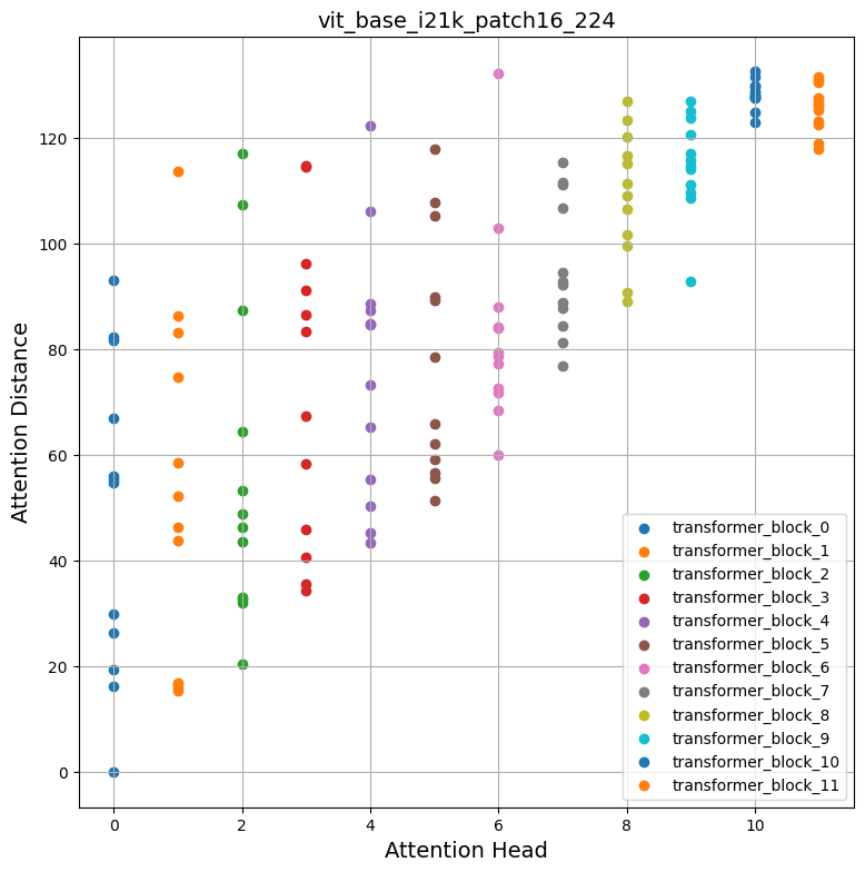
Attention is spread more widely over the image in later blocks, with the last 2–3 blocks effectively attending the entire image (mean attention distance is about half the image height/width). This is somewhat similar to the attention pattern of a CNN, which learns local features in the early layers and gradually builds longer-range features. However, the ViT has some long-range features even in the earliest Transformer blocks.
Key takeaways for class:
- Dual role in early blocks: In blocks 0–2, some attention heads exhibit very low attention distance (~20 pixels, comparable to a $5 \times 5$ conv kernel), acting as edge and texture detectors. Concurrently, other heads in the very same block have distances >80 pixels, attending across the full canvas.
- Convergence in late blocks: By blocks 9–11, almost all 12 heads have mean attention distances between 90 and 110 pixels (roughly half the $224\times 224$ image size, which is the expected average Euclidean distance between random pairs on a square). They integrate whole-object semantics.
- CNN contrast: A CNN is architecturally prevented from attending globally early on; ViT learns to do both simultaneously.
Cross-Image Invariance of Attention Distance
The graph above is based on a single image. Try generating this graph again for different images. Do you see changes in the attention pattern for different images/classes?
Cat image: Notice the characteristic bifurcation in early blocks (heads 1, 3 local vs heads 7, 10 global), smoothly narrowing to global coverage at block 11.
There is some variation, but most images should show very similar results.
Teaching notes:
- Architectural property: The mean attention distance curve is determined primarily by the trained weights $\mathbf{W}_Q, \mathbf{W}_K$ of the network, not the input pixels.
- Minor image shifts: Minor differences occur based on object scale (e.g. an extreme close-up of a dog face vs a small quokka in a field), but the overall trajectory from early local+global mixture to late purely-global attention remains invariant across natural images.
Attention Rollout: Walking the Residual Graph
Why can't we just look at the attention weights of the final layer to see what the model attended to?
Each Transformer block contains a skip connection: $\mathbf{x}_{l+1} = \mathbf{x}_l + f_{\text{attn}}(\mathbf{x}_l)$.
Because features flow through both the attention projection and the identity shortcut, information at layer $l+1$ is a combination of identity and attention. Abnar & Zuidema (2020) formulated Attention Rollout by combining the head-averaged attention $\mathbf{A}_l = \frac{1}{h}\sum_{k=1}^h \mathbf{A}_l^{(k)}$ with identity:
$$\hat{\mathbf{A}}_l = 0.5 \mathbf{A}_l + 0.5 \mathbf{I}$$Rollout recurses forward through the network depth as:
$$\tilde{\mathbf{A}}^{(l)} = \hat{\mathbf{A}}_l \cdot \tilde{\mathbf{A}}^{(l-1)}$$Expanding this recursion from layer 1 to layer $L$ yields the cumulative attribution matrix $\mathbf{R}$:
$$\mathbf{R}^{(L)} = \hat{\mathbf{A}}_L \cdot \hat{\mathbf{A}}_{L-1} \cdots \hat{\mathbf{A}}_1 \cdot \mathbf{I}$$(Notice that the matrices are left-multiplied in forward flow order $\hat{\mathbf{A}}_L \cdots \hat{\mathbf{A}}_1$, and the trailing $\cdot \mathbf{I}$ explicitly represents the base step $\tilde{\mathbf{A}}^{(0)} = \mathbf{I}$ so the sequence is crystal clear.) The first row $\mathbf{R}^{(L)}[0, 1:]$ gives the total cumulative attention from the [CLS] token to every image patch!
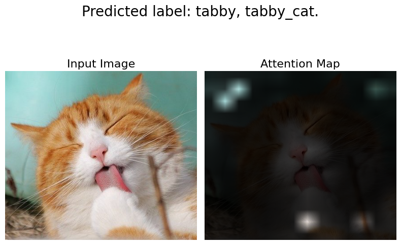
Notice how the attention rollout cleanly isolates the body, head, and ears of the cat while completely suppressing the background floor and furniture.
Attention Rollout vs. Head Specialization
Investigate how the attention pattern changes for (a) different images and (b) the final transformer layer versus an earlier one, and across individual attention heads.
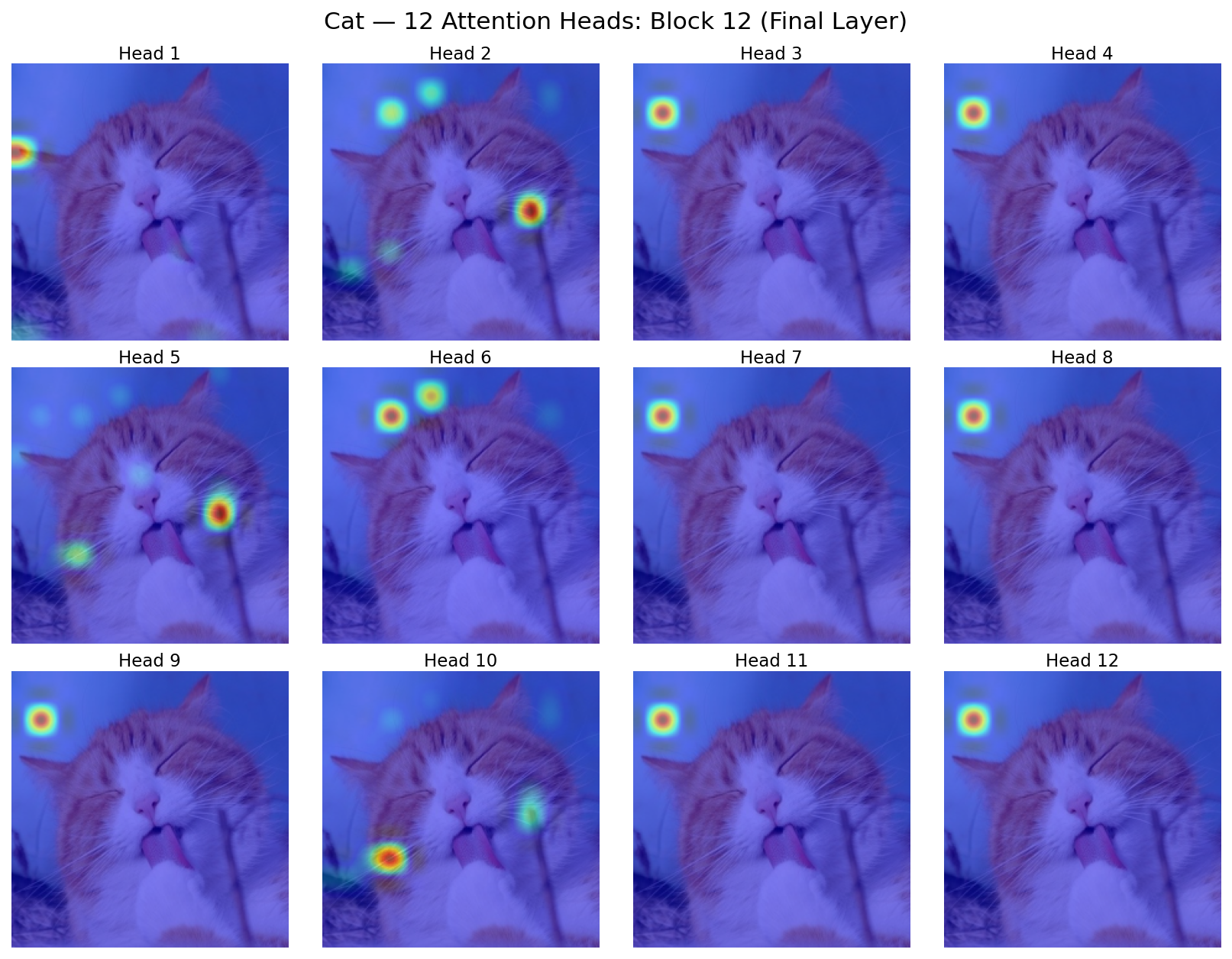
Generally, attention heads tend to specialise in detecting certain kinds of features, so different attention heads will have a stronger response to different images. As in a CNN, layers of a ViT attend to increasingly complex features. Attention heads in early Transformer blocks will generally show more diffuse attention because they attend to features that are present in many parts of an image (e.g., colours or shapes) while later blocks will attend to more object-specific features.
Teaching notes:
- Head specialization: Notice how Head 3 focuses sharply on the cat's face, while Head 5 isolates the whole animal body, and Head 9 focuses almost entirely on the surrounding context.
- Head pruning research: Pruning experiments (e.g. Voita et al., Michel et al.) show that up to 50–70% of attention heads can be removed at test time without catastrophic drop in accuracy, because multiple heads share redundant roles.
Grad-CAM 101: From Gradients to Heatmaps
How can we explain what a Convolutional Neural Network saw without changing the model or retraining?
Grad-CAM (Gradient-weighted Class Activation Mapping - Selvaraju et al., 2017) computes the gradient of the class score $y^c$ (before softmax) with respect to feature map activations $A^k$ of the final convolutional layer:
1. Neuron Importance Weights $\alpha_k^c$: Global Average Pool (GAP) the gradients over spatial dimensions width $u$ and height $v$ ($14 \times 14$):
$$\alpha_k^c = \overbrace{\frac{1}{Z}\sum_{i=1}^u \sum_{j=1}^v}^{\text{Global Average Pooling}} \frac{\partial y^c}{\partial A_{i,j}^k}$$where $Z = u \cdot v$ (for $14 \times 14$ feature maps, $Z = 14 \times 14 = 196$) is the spatial pixel count normalizing the average.
2. Rectified Weighted Combination: Take the weighted sum of forward feature maps and apply $\mathrm{ReLU}$:
$$L_{\text{Grad-CAM}}^c = \mathrm{ReLU}\left(\sum_{k=1}^K \alpha_k^c A^k\right)$$Target Class Disambiguation on Multi-Label Images
Explain how Grad-CAM behaves when an image contains multiple categories. For fruits.jpg, generate heatmaps for top-2 categories: "Granny Smith" (948) and "banana" (954).
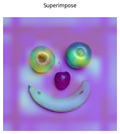
Notice how the Grad-CAM heatmap concentrates tightly on the green apples in the center and bottom, completely ignoring the bananas right next to them!
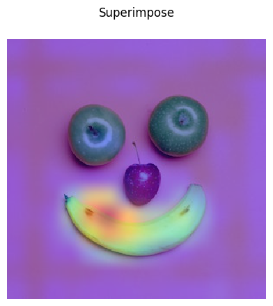
Grad-CAM enables class-discriminative visual explanations: targeting class 948 highlights the apples, while targeting class 954 highlights the bananas on the exact same input image.
Teaching notes & discussion:
- Class-discriminative power: Unlike basic saliency maps (which merely highlight all high-contrast edges in an image), Grad-CAM is strictly conditioned on the target class $c$.
- Failure cases / limitations: Grad-CAM's resolution is restricted by the feature map dimensions ($14 \times 14$ in VGG19's
block5_conv4). When multiple instances of the same object overlap, Grad-CAM will merge them into a single blob.
ViT Attention vs. CNN Grad-CAM: Comparative Matrix
How do the two explainability techniques compare in theory and in practice?
| Property | ViT Attention Rollout | CNN Grad-CAM |
|---|---|---|
| Core Mechanism | Intrinsic attention routing ($A_{i,j}$) & residual graph flow | Post-hoc backpropagated gradients ($\partial y^c / \partial A^k$) & GAP |
| Computational Cost | Free (calculated during standard forward pass) | Requires an extra backward pass per target class |
| Class Specificity | Input-dependent; reflects overall token routing | Strictly class-discriminative (different map per class $c$) |
| Spatial Resolution | $14 \times 14$ token grid ($16 \times 16$ px patches) | $14 \times 14$ conv feature map (upsampled to $224 \times 224$) |
| Supervision Needed | None (works directly on self-attention weights) | None (works directly on classification loss gradient) |
| Best Used For | Understanding internal token interactions & head specialization | Debugging false positive predictions & multi-label localization |