Arrays, plots
and pixels
Everything in this subject is a NumPy array wearing a costume.
Today we learn the array, how to look at it, and how to load one from a photograph.
numpy
·
matplotlib
·
cv2

Introduce yourself
Tell us your name, your course, and pick one:
Your name
What does your name mean, if you know?
Your background
What is your phone or laptop background?
A hobby
What do you enjoy doing when an assignment is not consuming your week?
Use the agent. Keep the understanding.
AI coding agents are excellent leverage. They are not a substitute for knowing what your program is doing.
Good work for an agent
- Boilerplate and repetitive edits
- Searching an unfamiliar codebase
- Explaining a new API or error message
- Reviewing a solution you can evaluate
Keep these skills yourself
- Read shapes, types and control flow
- Understand the snippets you submit
- Fix small bugs with prints and a debugger
- Code without assistance in interviews
Don’t burn tokens on a typo. Inspect the error, print the shape, read the docs, and use your brain before prompting an expensive model.
Four stops
NumPy
Create, inspect, slice, reshape and do arithmetic on n-dimensional arrays.
Matplotlib
Draw a labelled plot, and put several plots in one figure.
OpenCV
Read, display, crop, resize and write images — which are just arrays.
Exercise
Chain all three together, then a pinhole camera question.
By the end you should be able to look at img.shape and say out loud what every number means — and know the six mistakes that cost everyone an hour in Assignment 1.
One container, two lenses
Computer vision code is mostly moving numbers around. These libraries split that job cleanly:
- NumPy owns the data. A contiguous block of same-typed numbers, plus a shape describing how to read it.
- Matplotlib turns that data into something your eyes can check.
- OpenCV gets pixels in and out of files, and does the image-specific operations fast.
OpenCV does not invent its own image type. cv2.imread hands you a NumPy array, which is why everything you learn in the first half applies directly in the second.
The convention
import numpy as np
import matplotlib.pyplot as plt
import cv2
These three aliases are effectively universal. Use them — marker scripts and Stack Overflow answers both assume them.
Check your install
import sys; print(sys.version)
print(np.__version__, cv2.__version__)Creation · inspection · indexing · manipulation · operators
Building an array by hand
a = np.array([0, 1, 2, 3, 4])

b = np.array([[0, 1, 2, 3, 4],
              [5, 6, 7, 8, 9]], dtype=float)

c = np.array([[1, 6], [2, 7], [3, 8],
              [4, 9], [5, 10]], dtype=int)
Nested lists become extra dimensions. b is a list of two 5-element lists, so it is a 2×5 array. c is a list of five 2-element lists, so it is 5×2.
dtype fixes the type of every element. Unlike a Python list, an array cannot mix ints and strings — and that restriction is exactly what makes it fast.
b — shape (2, 5)
Axis 0 runs down the rows, axis 1 runs across the columns. Hold on to that — it decides what axis= means everywhere else.
c — shape (5, 2)
Arrays you ask for by shape
Most arrays in real code are not typed out. You declare a shape and let NumPy fill it.
size = (2, 3)

np.zeros(size)
np.ones(size)
np.full(size, 5)
np.empty(size)
np.eye(3)
np.random.random(size)
np.arange(1, 11)
np.linspace(0, 1, 5)
repr() in the worksheet is there so you can see the dtype and brackets, not just the pretty-printed numbers.
np.zeros | All 0.0 — the usual way to preallocate an output buffer. |
np.ones | All 1.0. Multiply by a constant for any fill value. |
np.eye(n) | Identity matrix. Takes one integer, not a shape tuple. |
np.full | Shape plus the value to repeat. |
np.random.random | Uniform on [0, 1). |
np.arange(a, b) | Evenly spaced values, stop excluded — like range. |
np.linspace | A fixed number of points between two ends, stop included — the sibling of arange. |
np.empty | Allocates memory without clearing it. Fast, but the contents are whatever was in RAM. Never read from it before you write to it. |
Four questions, four attributes
c.dtype   # int64   type of each element
c.shape   # (5, 2)  length of each dimension
c.ndim    # 2       number of dimensions
c.size    # 10      total number of elements
shape is the one you will type a hundred times this semester. ndim == len(shape) and size == prod(shape), always.
dtype=int means the platform default — int64 on Linux and macOS, int32 on Windows. Say np.int64 when the width has to be guaranteed.
Changing type
a.astype(np.float16)
b.astype(np.int8)      # 7.0 -> 7, truncates
astype returns a new array. Converting float to int truncates toward zero — it does not round.
Reading a shape
shape(2, 5) — 2 along axis 0, 5 along axis 1
ndim2
size10
dtypefloat64
Same five values, three different shapes
(5,) is the flat, one-dimensional array. Adding a length-1 axis makes a two-dimensional row or column.
a[2] → 2
A vector with five positions. It has no row or column orientation.
col[2, 0] → 2
Five rows and one column: a 2D column array.
row[0, 2] → 2
One row and five columns: a 2D row array.
a[:, np.newaxis] or a.reshape(5, 1)
creates the column shape.
a[np.newaxis, :] or a.reshape(1, 5)
creates the row shape.
[start : stop : step]
Stop is always excluded. Omit any part and NumPy fills in the default: start 0, stop the end, step 1. One slice per dimension, separated by commas.
b[0, 1]
a single element
a[0:4]
start:stop
a[0:4:2]
every second element
a[::-1]
a negative step walks backwards
b[:, 2]
every row, column 2
b[0, :3]
row 0, first three
A colon on its own means "all of this axis". You will write img[:, :, 0] constantly — every row, every column, channel 0.
It just quietly gives you less
Ask a slice for more elements than exist and NumPy hands back whatever it has. Only integer indexing raises.
a = np.arange(5)

a[0:100]         # array([0, 1, 2, 3, 4]) — no error
a[100]           # IndexError

a[2:100].shape # (3,) not 98 elementsNegative makes it worse
A negative index is not an error signal — it counts from the end. So arithmetic that should have been rejected produces a perfectly legal slice somewhere else in the array.
start = (5 - 9) // 2   # -2
a[start:start + 9]     # array([3, 4])
Nine elements were asked of a five-element array. The answer came back with two, taken from the opposite end.
When it bites: every "why is my array the wrong size" bug. The slice was legal — it just was not the one you meant. Any time a slice bound is computed rather than typed, this is live.
One line of insurance: assert out.shape == (9,) fails at the mistake instead of three cells later. You will see this exact arithmetic again in the OpenCV section.
Adding axes, and asking questions
np.newaxis
a.shape              # (5,)
a[:, np.newaxis].shape   # (5, 1)
Inserts a length-1 dimension. Turns a flat vector into a column vector so it will broadcast against a matrix. None works as a synonym.
Boolean indexing
a > 2        # [False False False  True  True]
a[a > 2]     # array([3, 4])
The comparison builds a mask of the same shape; indexing with it returns the elements where the mask is True — always as a flat 1D array.
Need the shape kept? np.where(a > 2, a, 0) chooses element-wise and hands back an array shaped like a.
Mask, then select
a
a > 2
a[a > 2]
This is how you will threshold an image: mask = img > 128 gives a boolean array the same size as the picture, and img[mask] = 255 edits only those pixels.
A slice is a window, not a photograph
Slicing an array gives you a view — a second way of looking at the same memory. Write through the view and the original changes underneath you.
b = np.array([[0,1,2,3,4],
              [5,6,7,8,9]], dtype=float)
row = b[0]        # a view, not a copy
row[0] = 99
print(b[0, 0])
The fix: make a copy
aa = a.copy()     # deep copy, independent memory
aa.fill(0)
print(a)
print(aa)
When it bites: you crop a region out of an image, adjust its brightness, and later discover the full-size image has a bright rectangle in it.
Rule of thumb: slicing and reshaping give views; fancy/boolean indexing, astype and arithmetic give new arrays. When in doubt, .copy() — it is cheap compared to the debugging.
Same numbers, different shape
b.ravel()            # -> (10,)   a view if it can
b.flatten()          # -> (10,)   always a copy
b.reshape(5, 2)      # -> (5, 2)
np.resize(b, (6,2))  # -> (6, 2)  b is (2, 5)
reshape vs resize
reshape keeps the element count fixed — it will raise an error if the new shape does not multiply out to size. np.resize will happily change the count, tiling the data to fill a bigger shape or truncating for a smaller one. The method b.resize(...) is a third thing again: in place, and it pads with zeros rather than tiling.
Use -1 for one dimension and NumPy infers it: b.reshape(-1, 2).
Reshape follows row-major order
Elements are read left-to-right, top-to-bottom, then poured into the new shape the same way. Nothing is sorted or transposed.
Adding and removing elements
b[0, :3] = 10            # assign into a slice, in place

np.append(a, [1, 1])     # values on the end
np.insert(a, 2, [1, 1])  # values at index 2
np.delete(a, [0, 2])     # drop indices 0 and 2
Assigning into a slice modifies the array you already have in place. The three functions do not — each returns a brand new array and leaves a untouched. If you do not capture the result, nothing happens.
Arrays have a fixed size in memory, so there is no cheap append. Growing an array in a loop copies the whole thing every iteration. Build a Python list and convert once, or preallocate with np.zeros and fill.
b[0, :3] = 10
One scalar on the right-hand side fills every selected cell. This is broadcasting, and it is how you will blank out a region of an image.
Stacking and splitting
np.concatenate((b, b+10), axis=0)   # (4, 5)
np.concatenate((b, b+10), axis=1)   # (2, 10)

np.r_[b, b+10]      # shorthand for axis=0
np.c_[b, b+10]      # shorthand for axis=1

np.split(b, 2, axis=0)   # list of 2 sub-arrays
axis=0 means "grow downward, along the rows". axis=1 means "grow sideways, along the columns". Every other axis must already match.
np.r_ and np.c_ use square brackets because they are indexing objects, not functions. Convenient, but spell out concatenate when the reader needs to see the axis.
axis = 0
(2,5) + (2,5) → (4,5)
axis = 1
(2,5) + (2,5) → (2,10)
Arithmetic is element-wise
a = np.array([0, 1, 2, 3, 4])
d = np.array([5, 6, 7, 8, 9])

a + d     # np.add
a - d     # np.subtract
a * d     # np.multiply
a / d     # np.divide
No loops. The operation is applied to every position independently and the result has the same shape.
* is not matrix multiplication — it multiplies element by element. For matrix products use @. This trips up people arriving from MATLAB.
Broadcasting
When shapes differ, NumPy stretches the smaller one if it can — comparing shapes from the right, dimensions must be equal or 1.
b + 10        # scalar reaches every element
b * np.array([1, 0, 0, 0, 1])
              # (2,5) * (5,) -> (2,5)
This is how you tint an image: multiply an (H, W, 3) array by a length-3 array of per-channel gains and every pixel gets scaled.
a / d promotes to float even when both inputs are integers. Use // if you want integer division — which matters when the result has to stay uint8.
Collapsing an array to a summary
b.sum()    # 45.0    everything
b.min()    # 0.0
b.max()    # 9.0
b.mean()   # 4.5
The axis argument
b.sum()          # 45.0   a scalar
b.sum(axis=0)    # [ 5.  7.  9. 11. 13.]
b.sum(axis=1)    # [10. 35.]
axis=k is the axis that disappears. Summing a (2, 5) array over axis 0 leaves shape (5,) — five numbers, one per column. Over axis 1 you get (2,), one per row.
Those trailing dots are not decoration — b was built with dtype=float, and the repr tells you so. Reading dtype off the output is a free habit.
Comparison
a == a     # [True True True True True]
b < 2      # a (2,5) array of booleans
Comparisons are element-wise too, so they give you an array — which means if a == b: raises "truth value of an array is ambiguous".
Comparing whole arrays
np.array_equal(a, b) # FalseReturns a single bool: same shape and same elements. For floats prefer np.allclose — exact equality after arithmetic is a coin toss.
Not the axis you keep
Almost everyone first reads axis=0 as "work along the rows". It means the opposite: axis 0 is collapsed, and everything else survives.
b.shape                # (2, 5)
b.sum(axis=0).shape    # (5,)   axis 0 is gone
b.sum(axis=1).shape    # (2,)   axis 1 is gone
Map it straight onto the shape tuple: axis=k deletes the k-th number from shape. That one sentence settles nearly every axis question you will have this semester.
On an image, both are legal
img.shape             # (512, 768, 3)
img.mean(axis=2)      # (512, 768)  grey per pixel
img.mean(axis=(0,1))  # (3,)  mean per channel
Both are "the mean of the image". They answer entirely different questions, and choosing wrong gives you a perfectly valid array instead of an error.
Note that axis=2 is not how you make a greyscale image. A flat mean gives every channel ⅓, but your eye weights them 0.299 R, 0.587 G, 0.114 B — so it triples blue's influence and nearly halves green's, which is the larger error. Use cv2.cvtColor(img, cv2.COLOR_BGR2GRAY).
Linear algebra
b.T                # transpose, (2,5) -> (5,2)
a.dot(a)           # dot product -> 30
b @ c              # (2,5) @ (5,2) -> (2,2)
x = c.T @ c
np.linalg.inv(x)   # inverse
b.trace()          # sum of the diagonal
np.eye(3)          # identity
Inner dimensions must agree: (2,5) @ (5,2) works, (2,5) @ (2,5) does not. Read the error message — it prints both shapes and tells you exactly which pair failed.
You will need this for homogeneous coordinates and camera matrices in a fortnight.
Universal functions
np.exp(a)
np.sin(a)
np.log(c)
np.abs(-b)
np.power(b, 3)
A ufunc applies a scalar function to every element and returns an array of the same shape — the same pattern as arithmetic, with a name.
Prefer np.log(x) over Python's math.log(x). The math module only accepts single numbers and will refuse an array.
Basic plots · subplots
A plot in six lines
x   = np.arange(-2, 2, 0.1)
y_1 = np.power(x, 2)
y_2 = -np.power(x, 2)

plt.plot(x, y_1, label=r'$x^2$')
plt.plot(x, y_2, label=r'$-x^2$')

plt.xlabel('x axis')
plt.ylabel('y axis')
plt.title('parabola')
plt.legend()
plt.show()
What each call does
plot | Draws a line through the (x, y) pairs. Call it again to add another line to the same axes. |
label= | Names the line. The r'...' raw string lets you write LaTeX maths between dollar signs. |
legend | Collects those labels into a box. Without labels it draws nothing. |
show | Renders the figure and closes it. The worksheet calls it twice — the second call finds nothing open and silently does nothing. |
This is the stateful interface: every call acts on the current figure. Fine for a worksheet. For anything you will reuse, fig, ax = plt.subplots() and calling methods on ax is easier to reason about.
One axis. Several Axes. Different ideas.
Memory line: a NumPy axis is a direction through data; a Matplotlib Axes is a drawing area. fig, ax = plt.subplots() returns one Figure and one Axes.
Several plots, one figure
plt.subplot(2, 1, 1)      # rows, cols, which
plt.plot(x, y_1)
plt.title(r'$x^2$')

plt.subplot(2, 1, 2)      # now the second panel
plt.plot(x, y_2)
plt.title(r'$-x^2$')

plt.tight_layout(pad=2.0)
plt.show()
subplot(nrows, ncols, index) selects a cell in a grid and makes it the active axes. Everything you draw afterwards lands there until you select another.
The index starts at 1, not 0 — the one place in this workshop where you do not count from zero. It runs left to right, then top to bottom.
tight_layout pushes the panels apart so titles and tick labels stop overlapping.
subplot(2, 2, k)
You need exactly this 2×2 grid for the exercise.
Read · show · crop · resize · write
An image is an ndarray
import os
rootpath = './'
path = os.path.join(rootpath, "kodim23.png")
bird = cv2.imread(path)

type(bird)
bird.shape
bird.dtype512rows — the height, axis 0
768columns — the width, axis 1
3colour channels, axis 2
uint8each value is an integer 0–255
Row before column. The origin is the top-left corner and the row index increases downward — the opposite of a maths y-axis.
cv2.imread(path, cv2.IMREAD_GRAYSCALE) returns a 2D (512, 768) array instead — one channel, no axis 2 at all.
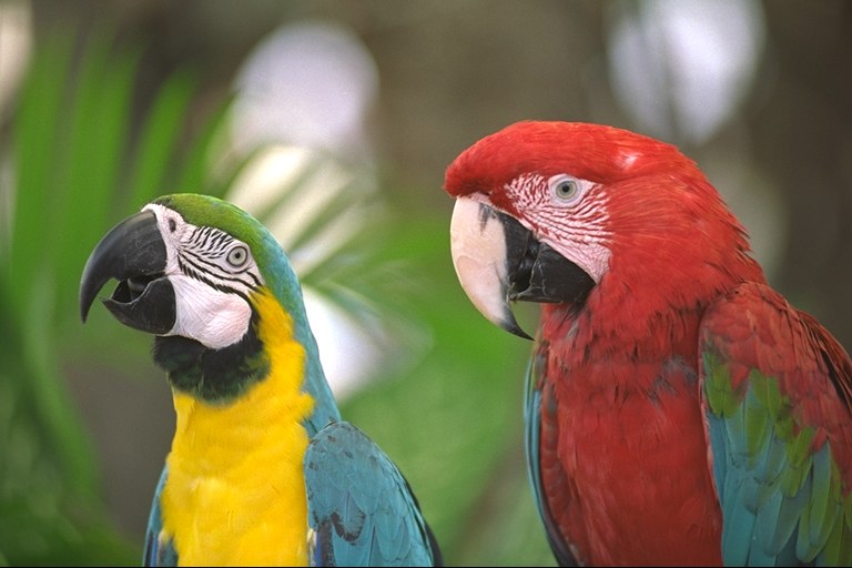
kodim23.png — 768 wide, 512 high → shape (512, 768, 3)
(H, W, C)
Height and width are the two directions within every colour plane. The three planes are stacked along axis 2.
This photograph is 3,686,400 numbers
bg = cv2.imread("my-bg.jpeg")

bg.shape
bg.dtype
bg.size
The skyline, clouds, people and bright sunset reflection are not separate objects to NumPy. They are just rows, columns and three channel values.
At roughly bg[350, 650], OpenCV sees three BGR numbers. We see sunset reflected in glass. Computer vision is the work required to bridge those two descriptions.
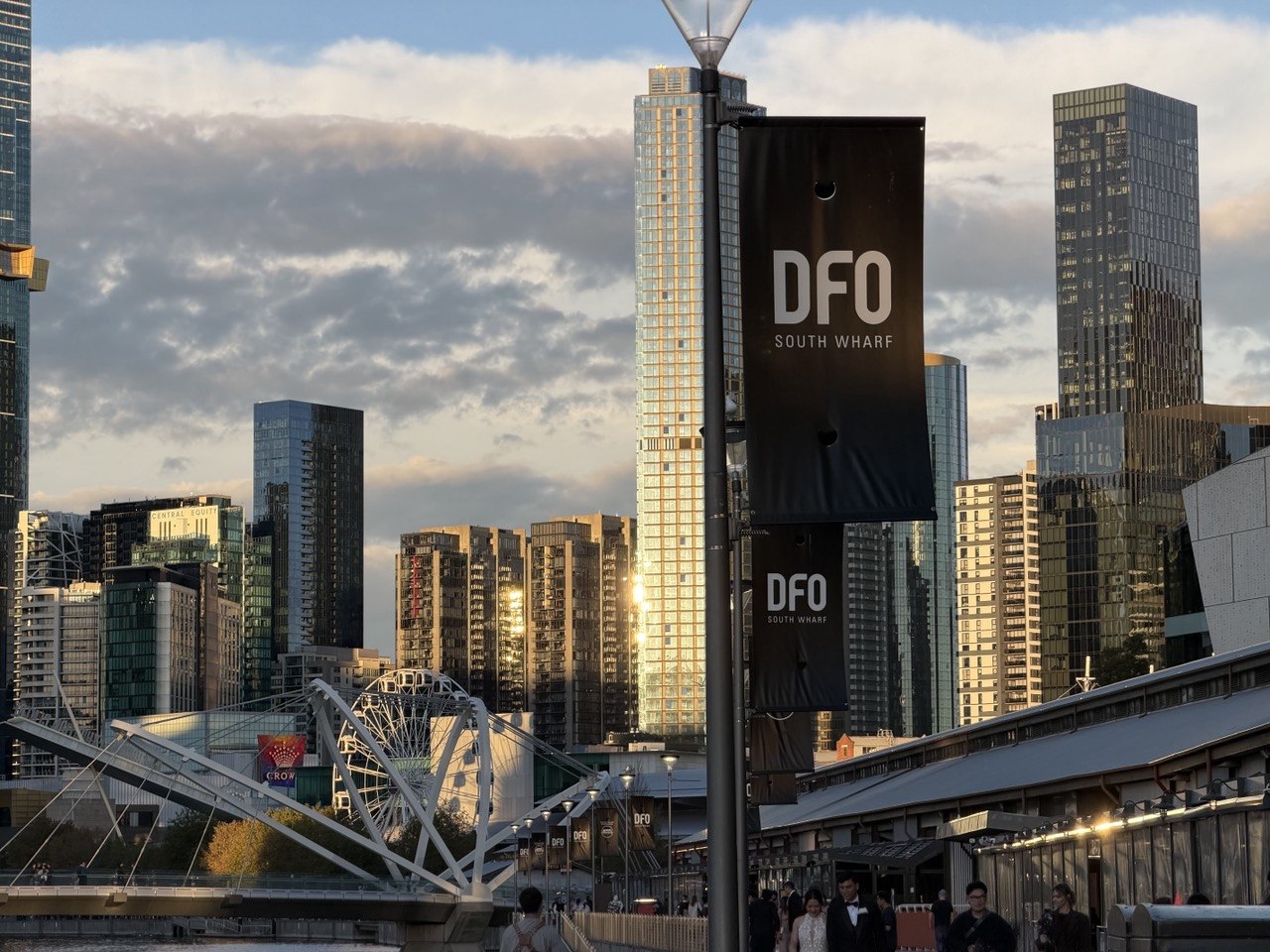
(row, column, channel) = (y, x, BGR). The origin is the top-left corner.
Why your photo looks like a Martian sunset
cv2.imread returns channels in blue, green, red order. plt.imshow assumes red, green, blue. Hand one to the other and red and blue trade places. Nothing errors — the array is valid and the shape is right.
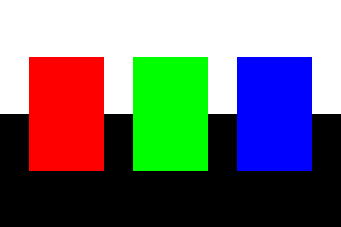
cvtColor — correct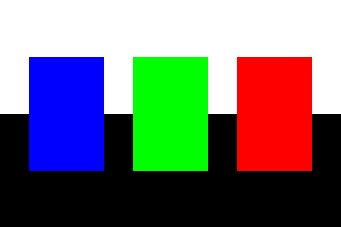
plt.imshow(rgb_test) — red and blue swappedThe white and green bars are identical in both. Only the two ends move — which is exactly why the bug survives a glance at a photograph.
Two ways out
rgb_test  = cv2.imread("rgbtest.png")   # BGR!
image_rgb = cv2.cvtColor(rgb_test, cv2.COLOR_BGR2RGB)
plt.imshow(image_rgb)                   # now correct
The worksheet's variable name lies to you. rgb_test holds BGR data — it is named after the file, not its contents. image_rgb is the one that is actually RGB. Name arrays after what is in them.
…or wrap it once and never think about it again:
def imshow(image, *args, **kwargs):
  if len(image.shape) == 3:
    image = cv2.cvtColor(image, cv2.COLOR_BGR2RGB)
  else:
    image = cv2.cvtColor(image, cv2.COLOR_GRAY2RGB)
  plt.imshow(image, *args, **kwargs)
  plt.axis('off')
  plt.show()
The grayscale branch matters too: a 2D array sent to imshow is drawn with a false-colour map, not in black and white.
Interrogating pixels
image_rgb[100, 100, :]   # [255   0   0]  red
image_rgb[100, 200, :]   # [  0 255   0]  green
image_rgb[100, 300, :]   # [  0   0 255]  blue
image_rgb[  0,   0, :]   # [255 255 255]  white
image_rgb[226, 340, :]   # [  0   0   0]  black
Row first, then column, then channel — the same order as shape. White is all channels at maximum, black is all at zero.
This is the check to run whenever you are unsure which convention an array is in. Point at a pixel whose colour you already know and read the numbers.
One channel at a time
imshow(bird[:, :, 0])   # blue  (BGR!)
imshow(bird[:, :, 1])   # green
imshow(bird[:, :, 2])   # red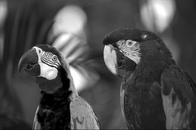
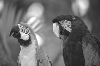
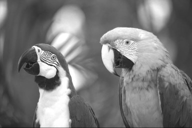
Each is a 2D array shown in grayscale — lighter means a higher value. Look at the sky: bright in blue, dark in red. Indexing with an integer drops the channel axis, so bird[:,:,0].shape is (512, 768), which is why the helper has a grayscale branch.
Cropping is just slicing
crop_1 = bird[150:500, 50:350, :]Rows 150–499, columns 50–349, all channels. There is no cv2.crop — you already know how to do this.
Centre crop
def crop_center(image, crop_size):
    height = image.shape[0]
    width  = image.shape[1]
    upper_crop = (height - crop_size) // 2
    left_crop  = (width  - crop_size) // 2
    return image[upper_crop:upper_crop + crop_size,
                 left_crop:left_crop + crop_size, :]
Halve the leftover margin to find the top-left corner, then take crop_size from there. // keeps the result an integer — array indices cannot be floats.
image[y0:y1, x0:x1]
Rows are the first slice. Put the x range first and you still get a crop — just not the one you meant, and still without an error.
Trap 1, in the wild
crop_center(bird, 500)  # (500, 500, 3)
crop_center(r224, 500)  # (138, 138, 3) ???
r224 is the 224×224 resize, so the offset is (224 - 500) // 2 = -138 — trap 1's computed negative bound. It wraps to row 86 and the crop lands 138 square. No guard, no error.
The exercise needs different width and height, so crop_center needs two size arguments. Work out which line each belongs to.
Subtract the crop, then split the leftover space
For the exercise, the image is 224 pixels high and the crop should be 156 pixels high. A centred crop needs equal margins above and below.
After reserving 156 rows for the crop, 68 rows remain outside it.
Split those leftover rows equally: 34 above and 34 below.
image[34 : 34 + 156] takes rows 34–189.
The same reasoning horizontally leaves 48 columns on each side.
224 × 224 image → 156 × 128 crop
Memory rule: subtraction finds the total leftover border; dividing by two finds the starting index for a centred crop.
Same photo. Different protagonist.
# Skyline and ferris wheel
city = bg[294:900, 0:650, :]

# Isolate the sunset reflection
reflection = bg[56:812, 590:770, :]
A crop is not only a smaller array. It changes what the image appears to be about. Coordinates are a creative decision as well as a technical one.
Debugging clue: these crops have different aspect ratios. If a supposedly wide skyline comes out tall, the row and column ranges were probably swapped.
The one that flips your image
shape gives (height, width). cv2.resize takes (width, height) — the opposite order. Read the shape tuple, hand it straight to resize, and you have transposed the picture.
img.shape             # (300, 400, 3)

wrong = cv2.resize(img, (300, 400))
wrong.shape           # (400, 300, 3)  flipped
The shape tuple went straight in, so resize read 300 as the width and 400 as the height. A 300×400 image came back standing on its end — and no exception, because that is what it was asked for.
h, w = img.shape[:2]
right = cv2.resize(img, (w, h))   # width first
Why it hides
On a square image the two orders are identical, so it works on your test picture and fails on the real dataset. On a non-square image you get a valid, wrongly-proportioned result and no error at all.
Habit worth forming: after every resize, print out.shape and check it against what you asked for. Two seconds now, an hour saved later.
The exercise's 224×224 target is square, so it will not catch this. The 128×156 crop is not — that one will.
Choosing how to invent pixels
h, w, c = rgb_test.shape
new_h, new_w = h // 10, w // 10

img1 = cv2.resize(rgb_test, (new_w, new_h),
                  interpolation=cv2.INTER_NEAREST)
img2 = cv2.resize(rgb_test, (new_w, new_h),
                  interpolation=cv2.INTER_CUBIC)
The output grid rarely lines up with the input grid, so every output pixel sits between input pixels. The interpolation flag decides what value it gets.
INTER_NEAREST | Copy the closest input pixel. Fast, blocky, and the only safe choice for label masks — it never invents a value that was not there. |
INTER_LINEAR | Weighted average of 4 neighbours. The default. |
INTER_CUBIC | Fits a cubic over 16 neighbours. Smoother, slower, can overshoot slightly at edges. |
INTER_AREA | Averages over the source region. Best for shrinking. |
Where the difference shows
NEAREST
CUBIC
The worksheet shrinks by 10× and then the browser scales the result back down, so the two look nearly identical. To see the real difference, upsample a small crop instead.
Pixelated on purpose; colour-swapped by mistake
# Pixel-art Melbourne — 20x down, then 16x back up
tiny = cv2.resize(bg, (64, 48),
                  interpolation=cv2.INTER_AREA)
pixelated = cv2.resize(
    tiny, (1024, 768),
    interpolation=cv2.INTER_NEAREST)

# Accidental BGR-as-RGB display
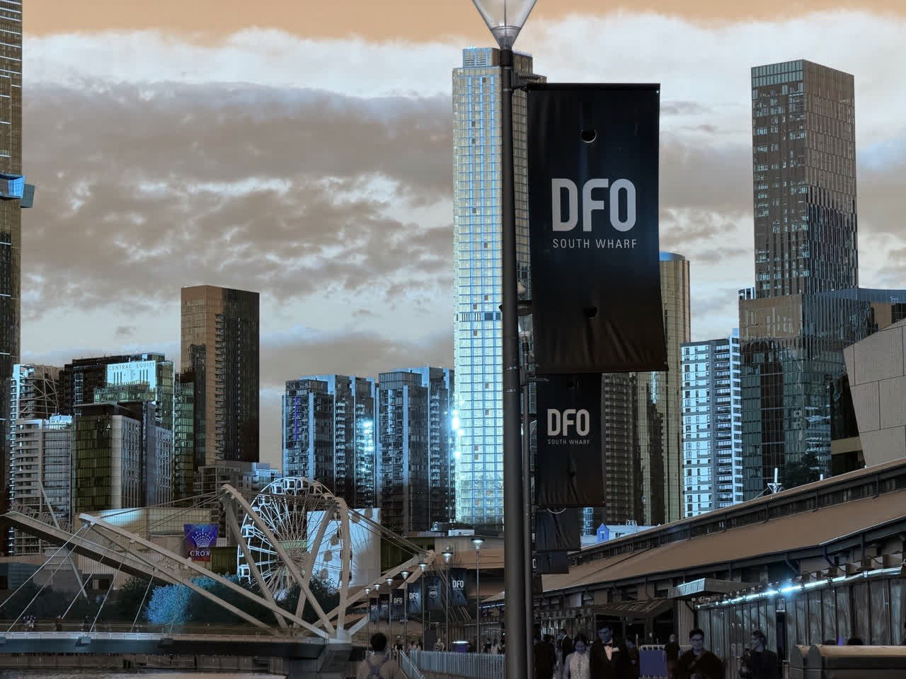
plt.imshow(bg)  # forgot cvtColor!
Compare the first two panels: the original has the correct colour, while the BGR-as-RGB version swaps red and blue. The third throws away spatial detail on purpose.
1280/20 = 64 and 960/20 = 48, so the 4:3 shape survives. Pick (64, 40) instead and you have quietly squashed the picture — trap 5, wearing a different hat.
Why the error is easy to miss: this photograph has muted colours, so the swapped version remains plausible. Look at the golden reflection becoming cold and the blue-grey sky shifting warmer. A valid shape is not proof of correct colour.

Getting pixels back out
out = os.path.join(rootpath, "resize_bird.jpeg")
cv2.imwrite(out, resize_img3)

test = cv2.imread(out)
print(test.shape, test.dtype)
imshow(test)
The file extension picks the encoder — .png, .jpeg, .tif. There is no format argument.
imwrite expects BGR, the same order imread gave you. If you converted to RGB for display, convert back before saving or your saved file will have the channels swapped.
Round-trip is not always lossless
JPEG is lossy: write then read and the pixel values shift slightly. PNG is lossless.
For intermediate results you will compute on — masks, depth maps, anything you compare numerically — save as PNG. Save JPEG only for the final picture a human looks at.
It returns a bool
imwrite returns False rather than raising when the directory does not exist — so if your file never appears, check the return value. An unknown extension is different: that raises cv2.error outright.
Where the bright speckles come from
An image is uint8. Every value gets exactly 8 bits, and NumPy will not widen the type to fit your answer — it wraps.
green = np.uint8([200])
blue  = np.uint8([180])

green + blue
(green + blue) // 2
No warning, no error. Averaging two bright pixels hands back a dark one, so the damage lands exactly where the picture was brightest.
Widen, compute, come back
wide = green.astype(np.uint16)
avg = (wide + blue) // 2
red = avg.astype(np.uint8)
Anything that can leave 0–255 — brightening, scaling contrast, differencing two frames — needs clipping before the cast back:
out = np.clip(x, 0, 255).astype(np.uint8)When it bites: step 4 of today's exercise, the moment you reach for (g + b) // 2.
The mirror image: plt.imshow reads uint8 as 0–255 but float as 0–1. Cast to float for arithmetic, forget to divide by 255, and every pixel clips to pure white. Matplotlib logs one line about it that nobody notices.
Read · resize · crop · recolour · plot — then one pinhole camera
Put it together
- Read the bird image.
- Resize to 224×224 with bicubic interpolation.
- Centre-crop it — 128 wide, 156 high.
- Set the red channel to the mean of the green and blue channels, per pixel.
- Show all four images in a 2×2 subplot grid.
bird = cv2.imread(...)                 # 1
resized = cv2.resize(...)              # 2
cropped = crop_center(...)             # 3

recoloured = cropped.copy()            # 4  why .copy()?
recoloured[:, :, ?] = ...

plt.subplot(2, 2, 1)                   # 5
imshow(...)   # careful: imshow() calls plt.show()
Hints
- Step 3:
crop_centeras written takes one size. You need two. - Step 4: which index is red? The array came from
imread, so check the channel order before you pick. - Step 4:
uint8 + uint8wraps at 255 — trap 6. Adding first is what wraps;g/2 + b/2promotes to float and survives, and so does widening touint16. Both work — know which one you wrote. - Step 5: the helper
imshowends withplt.show(), which closes the figure. For a grid, callplt.imshowyourself on RGB-converted arrays andplt.show()once at the end. Open withplt.figure(figsize=(9,7))or four panels come out unreadably small.
Check yourself
Print .shape and .dtype after each step: (512,768,3) → (224,224,3) → (156,128,3), uint8 the whole way. Last shape reads (128,156,3)? Trap 5. Smaller than that? Trap 1. Speckles in the recoloured panel? Trap 6.
What Python is actually telling you
Each of these has one boring cause. Learning the mapping is most of what "getting good at debugging" means in this subject.
Jupyter is running a different interpreter to the one you installed into. Relaunch from the CV environment; print(sys.version) tells you which one you are on.
cv2.imread could not find the file, so it returned None. Your path is wrong — the error surfaces a line or two after the actual mistake.
You wrote img.shape(0). shape is a tuple, not a method: img.shape[0].
A / where you needed //. Array indices cannot be floats, even whole-numbered ones.
cv2.resize was handed a float size — same cause. Write w // 10, not w / 10.
You wrote if a == b:. The comparison returns an array, not a bool. Use np.array_equal, or .any() / .all().
reshape must preserve the element count, and 3×4 is not 10. Check .size, or pass -1 for one dimension.
The inner dimensions of @ disagree. (2,5) @ (5,2) works; (2,5) @ (2,5) does not. The message prints both shapes.
cv2.imwrite does not recognise your file extension. Use .png, .jpeg or .tif — the extension is what picks the encoder.
You called cv2.imshow in a notebook. It opens a native window and blocks until waitKey; Colab disables it outright. Use the imshow helper from the worksheet instead.
Six things that will bite you
1 · Slice bounds
An over-long slice does not raise — it returns fewer elements, and negative indices wrap. Assert the shape you expect.
2 · Views
A slice shares memory with its parent. Edit the crop, edit the original. .copy() when you mean a copy.
3 · axis=
The axis you name is the one that disappears. Row = axis 0 = the first number in shape.
4 · BGR
imread gives BGR, plt.imshow expects RGB. No error, just wrong colours. Convert once, at the boundary.
5 · (w, h)
shape is (rows, cols); resize takes (width, height). Print the shape afterwards, every time.
6 · uint8 wraps
Pixel arithmetic overflows silently at 255 and wraps to 0. Widen before you add, clip, then cast back.
The habit that covers most of them
After every operation, print shape and dtype. Traps 1, 3 and 5 show up in shape; 6 is the one dtype warns you about before it happens; 4 you can see. Views is the one that shows up in neither — the shape is right, the dtype is right, and the numbers quietly changed somewhere else. That is why .copy() is a habit rather than a check.
NumPy
- NumPy: the absolute basics for beginners — the official starting point.
- Scientific Python Lectures, NumPy chapter — covers today's material in more depth. CC BY 4.0.
- Rougier, NumPy tutorial — excellent diagrams for slicing. CC BY-SA 4.0.
- 100 NumPy exercises — practice, with solutions. MIT.
- Stanford CS231n Python/NumPy tutorial — the best short explanation of broadcasting.
Matplotlib
- Official cheatsheets — print the beginner handout and keep it next to you.
- Quick start guide — figure and axes explained properly.
Images
- OpenCV-Python tutorials — the reference for every function used today.
- Data Carpentry: Image Processing with Python — pixels, coordinates and colour models from scratch. CC BY 4.0.
Diagrams in this deck are original. Course content follows the COMP90086 Workshop 2 worksheet.