Cell 2Pin scikit-image (Colab)
## For colab user, run
! pip install scikit-image==0.21.0
## After the update, You must restart the runtime in order to use newly installed versions.A primer on lectures 19 and 20, then the Workshop 11 notebook cell by cell. Every algorithm the notebook calls from a library also runs live on this page.
Segmentation assigns a label to every pixel.
The lectures distinguish problems by what that label means:
Slide 41 adds the vocabulary for this split. Things are countable objects (cow, person, car). Stuff is regions or materials (road, grass, sky).2 Instance segmentation focuses on things.
The simplest segmenter ignores where pixels are and looks only at their colour.
Each pixel becomes a point in colour space, for example \((R, G, B)\) or \((L, a, b)\). Clusters of points become segments.
k-means looks for \(k\) centres \(\boldsymbol\mu_1, \dots, \boldsymbol\mu_k\) and an assignment \(c_i\) of each point that minimise the within-cluster sum of squares:3
$$J = \sum_{i=1}^{n} \big\lVert \mathbf x_i - \boldsymbol\mu_{c_i} \big\rVert^2 .$$Lloyd's algorithm alternates two steps until nothing changes:
Assignment step. Each term \(\lVert\mathbf x_i - \boldsymbol\mu_{c_i}\rVert^2\) is replaced by the smallest of its \(k\) options, so no term grows.
Update step. With the assignments fixed, consider one cluster \(S\). Its contribution, as a function of a single centre \(\boldsymbol\mu\), is
$$J_S(\boldsymbol\mu) = \sum_{i \in S} \lVert \mathbf x_i - \boldsymbol\mu \rVert^2 .$$Setting the derivative to zero gives the minimiser:
$$\frac{\partial J_S}{\partial \boldsymbol\mu} = -2\sum_{i\in S}(\mathbf x_i - \boldsymbol\mu) = 0 \quad\Longrightarrow\quad \boldsymbol\mu = \frac{1}{|S|}\sum_{i \in S}\mathbf x_i .$$So moving the centre to the mean can only lower \(J_S\).
\(J \ge 0\), it never increases, and there are finitely many assignments, so the algorithm stops. It stops at a local minimum, not necessarily the global one.
Slide 12 replaces hard assignments with a Gaussian mixture model. Each cluster becomes a Gaussian with its own covariance, and each pixel gets a probability of belonging to each cluster. k-means is the limiting case where every cluster has the same tiny spherical covariance.
Mean shift treats the points as samples from an unknown probability density, and looks for its peaks (modes).4
Each point is then labelled by the peak it climbs to. The number of clusters is not chosen in advance: it is the number of peaks.
The procedure on slide 24 is:
The move from \(\mathbf x\) to the weighted mean is the mean-shift vector (slide 23). The weights come from a kernel profile \(g\):
$$\mathbf m(\mathbf x) = \frac{\displaystyle\sum_{i=1}^{n} \mathbf x_i\, g\!\left(\left\lVert \frac{\mathbf x - \mathbf x_i}{h}\right\rVert^2\right)}{\displaystyle\sum_{i=1}^{n} g\!\left(\left\lVert \frac{\mathbf x - \mathbf x_i}{h}\right\rVert^2\right)} - \mathbf x .$$A flat kernel gives \(g = 1\) inside the window and \(0\) outside, so the update is the plain mean of the points in the window. A Gaussian kernel weights every point by its distance, with \(g(u) = e^{-u/2}\).
A kernel density estimate puts a bump of width \(h\) on every point. With profile \(k\):
$$\hat f_h(\mathbf x) = \frac{C}{n}\sum_{i=1}^{n} k\!\left(\left\lVert \frac{\mathbf x - \mathbf x_i}{h}\right\rVert^2\right).$$Differentiate with the chain rule, and write \(g = -k'\):
$$\nabla \hat f_h(\mathbf x) = \frac{2C}{nh^2}\sum_{i=1}^{n} (\mathbf x_i - \mathbf x)\, g\!\left(\left\lVert \frac{\mathbf x - \mathbf x_i}{h}\right\rVert^2\right).$$Pull out the sum of the weights \(g_i\):
$$\nabla \hat f_h(\mathbf x) = \frac{2C}{nh^2}\Big(\sum_{i} g_i\Big)\left[\frac{\sum_i \mathbf x_i g_i}{\sum_i g_i} - \mathbf x\right] = \frac{2C}{nh^2}\Big(\sum_{i} g_i\Big)\, \mathbf m(\mathbf x).$$The bracket is exactly the mean-shift vector. So \(\mathbf m(\mathbf x)\) always points uphill on \(\hat f_h\), and the window stops where the gradient is zero: at a peak.
For the Gaussian profile \(k(u) = e^{-u/2}\), we get \(g(u) = \tfrac12 e^{-u/2}\), again Gaussian. The flat window corresponds to the Epanechnikov profile \(k(u) = 1 - u\) for \(u \le 1\), whose derivative is constant inside the window.
Clustering in colour and position. Slide 25 appends the pixel coordinates to the colour, giving five-dimensional features \((x, y, L, a, b)\).
Each dimension has its own bandwidth, or equivalently, the coordinates are rescaled before one shared bandwidth is used (the notebook does this in cell 25). A larger spatial bandwidth relative to the colour bandwidth gives smoother, more blob-like regions (slide 26).
Over-segmentation splits the image into regions that are smaller than objects. Objects are still separated from the background, but each object is broken into many parts.
These parts are superpixels: groups of adjacent pixels with similar colour. They make a compact intermediate representation: a \(600 \times 800\) image of \(480\,000\) pixels becomes about \(200\) superpixels (slide 35).
SLIC (simple linear iterative clustering) is k-means in \((l, a, b, x, y)\) space with two changes:5
The distance mixes colour and position (slide 32):
$$D = d_{lab} + \frac{\alpha}{S}\, d_{xy},$$ $$d_{lab} = \sqrt{(l - l_k)^2 + (a - a_k)^2 + (b - b_k)^2}, \qquad d_{xy} = \sqrt{(x - x_k)^2 + (y - y_k)^2}.$$The weight \(\alpha\) is the compactness. A large \(\alpha\) gives regular, grid-like cells. A small \(\alpha\) lets cells follow colour edges closely.
Superpixels are usually a first step. To find whole objects, neighbouring superpixels with similar colour are merged.
The region adjacency graph (RAG) organises this:
Iterative merging (slide 36) repeats one move:
Merging builds regions bottom-up. A cut works top-down: split the graph into two sets \(A\) and \(B\) by deleting edges.
Here edge weights measure similarity (large means alike). The cost of a split is the weight of the deleted edges:
$$\operatorname{cut}(A, B) = \sum_{i \in A,\ j \in B} w_{ij}.$$The minimum cut has a flaw: cutting off one weakly connected node is cheap, so it favours tiny segments.
The normalised cut fixes this by dividing by each side's total connection to the whole graph, \(\operatorname{assoc}(A, V) = \sum_{i \in A} d_i\), where \(d_i\) is the weighted degree of node \(i\):6
$$\operatorname{Ncut}(A, B) = \frac{\operatorname{cut}(A, B)}{\operatorname{assoc}(A, V)} + \frac{\operatorname{cut}(A, B)}{\operatorname{assoc}(B, V)} .$$A tiny \(A\) has a tiny \(\operatorname{assoc}(A, V)\), so its first term is large. Balanced splits along weak edges score best.
Trying every split is exponential in the number of nodes. Shi and Malik relax the binary labels to real numbers. The relaxed problem becomes a generalised eigenvalue problem with the degree matrix \(D\) and the weight matrix \(W\):
$$(D - W)\,\mathbf y = \lambda D\, \mathbf y .$$The eigenvector with the second-smallest eigenvalue is thresholded to give the split, and splitting is applied recursively. skimage.graph.cut_normalized does this on the superpixel RAG of cell 37.
Clustering finds colour regions, and those regions often do not correspond to objects (slide 27).
The standard approach to instance segmentation (slide 42) has two stages:
Slide 43 gives two examples:
GrabCut minimises an energy over the labels \(\alpha_p \in \{\text{fg}, \text{bg}\}\):
$$E(\boldsymbol\alpha) = \underbrace{\sum_{p} -\log p\big(\mathbf z_p \mid \alpha_p\big)}_{\text{colour likelihood}} \; + \; \lambda \underbrace{\sum_{(p,q)\ \text{neighbours}} [\alpha_p \ne \alpha_q]}_{\text{boundary length}} .$$It alternates between refitting the two colour models and relabelling the pixels, and the energy falls at every round (slide 47).
Lecture 20 turns to methods that use labels. The first idea (slide 8) is to classify every pixel from an \(N \times N\) window around it.
Run naively, that is one CNN evaluation per pixel: \(480\,000\) evaluations for a small \(600 \times 800\) image (slide 9).
A fully-convolutional network (FCN) has no fully-connected layers. It produces a spatial map of class scores in one pass, so it classifies all windows in parallel and accepts any input size (slides 10–11).9
Slide 12 names two problems with a plain stack of convolutions:
The solution is an encoder–decoder (slide 13): the encoder downsamples, and the decoder upsamples back to \(H \times W\).
Let \(r_\ell\) be the receptive field after layer \(\ell\), and \(j_\ell\) the distance in input pixels between neighbouring units of layer \(\ell\) (the product of the strides so far). Start from \(r_0 = 1\) and \(j_0 = 1\).
A layer with kernel size \(k\) and stride \(s\) adds \(k - 1\) units of the layer below, and each of those spans \(j_{\ell-1}\) input pixels:
$$r_\ell = r_{\ell-1} + (k - 1)\, j_{\ell-1}, \qquad j_\ell = j_{\ell-1}\, s .$$For \(3 \times 3\) convolutions with stride 1, every step adds 2, so \(r_L = 2L + 1\): linear growth.
A \(2 \times 2\) pooling layer adds \(j_{\ell-1}\) and doubles \(j\). After that, the next convolution adds twice as much, which is why the growth becomes geometric.
The decoder needs layers that make feature maps larger. Lecture 20 gives two.
Each upsampling layer is paired with a max-pooling layer in the encoder (slide 15).10
The simpler alternatives on slide 14 copy each value into the whole block (nearest neighbour) or always into the top-left corner (bed of nails).
A convolution with stride 2 is a learnable downsampler: the filter moves 2 pixels in the input for every 1 pixel in the output (slide 18).
A transposed convolution reverses the roles. The filter moves 2 pixels in the output for every 1 pixel in the input:
Some papers call this "deconvolution", "upconvolution" or "fractionally strided convolution".11
Slides 23–24 write convolution as a matrix product. For kernel \(\vec x = [x, y, z]\), stride 2 and padding 1, convolving a length-4 signal \(\vec a\) (padded to length 6) is
$$\vec x * \vec a = X \vec a = \begin{bmatrix} x & y & z & 0 & 0 & 0 \\ 0 & 0 & x & y & z & 0 \end{bmatrix}\begin{bmatrix} 0 \\ a \\ b \\ c \\ d \\ 0 \end{bmatrix} = \begin{bmatrix} ay + bz \\ bx + cy + dz \end{bmatrix}.$$The transposed convolution multiplies by the transpose of the same matrix. A length-2 input becomes a length-6 output, two of which are padding:
$$\vec x *^{T} \vec a = X^{T} \vec a = \begin{bmatrix} x & 0 \\ y & 0 \\ z & x \\ 0 & y \\ 0 & z \\ 0 & 0 \end{bmatrix}\begin{bmatrix} a \\ b \end{bmatrix} = \begin{bmatrix} ax \\ ay \\ az + bx \\ by \\ bz \\ 0 \end{bmatrix}.$$Read down a column of \(X^{T}\): it is the kernel, shifted by the stride. That is exactly the "stamp and add" rule above.
Let \(\mathbf u = X\mathbf a\) be a strided convolution and \(L\) any loss. By the chain rule:
$$\frac{\partial L}{\partial a_j} = \sum_i \frac{\partial L}{\partial u_i}\,\frac{\partial u_i}{\partial a_j} = \sum_i X_{ij}\,\frac{\partial L}{\partial u_i} \quad\Longrightarrow\quad \nabla_{\mathbf a} L = X^{T}\, \nabla_{\mathbf u} L .$$So a transposed convolution is the operation that carries gradients back through a strided convolution. It maps a short vector back to the long one, which is why it upsamples. It is not the inverse of the convolution: \(X^{T}X \ne I\) in general.
The last layer. A \(1 \times 1\) convolution mixes channels at each pixel without looking at neighbours. With \(C\) output channels it turns every pixel's feature vector into \(C\) class scores (slide 26).
The loss. Training compares the predicted class distribution \(\hat{\mathbf y}_p\) with the true class at every pixel \(p\), and averages the cross-entropy over the \(N\) pixels (slide 27):
$$E = -\frac{1}{N}\sum_{p=1}^{N} \sum_{c=1}^{C} y_{p,c}\, \log \hat y_{p,c} .$$U-Net was built for biomedical images.12 It is an encoder–decoder with one extra idea: each decoder stage concatenates the upsampled map with the feature map from the matching encoder stage (slides 33–34).
The encoder copy carries fine spatial detail that pooling threw away, and the decoder supplies context. For cell segmentation, U-Net also weights the loss so that the thin gaps between touching cells count more.
The original network uses unpadded ("valid") \(3 \times 3\) convolutions, so each one shrinks the map by 2 pixels. The encoder maps are cropped before they are concatenated, which is the "copy and crop" arrow.
The Segment Anything Model (SAM) takes an image plus a prompt and returns a binary mask (slide 38).13 A prompt can be a point, a box, a mask or a text embedding.
Its encoder–decoder structure (slides 39–41) has three parts:
Ambiguity. A point on a person's shirt could mean the shirt or the whole person. SAM outputs three masks (for example subpart, part and whole), and is trained by back-propagating only the best of the three (slide 42).
Training. The mask loss combines focal loss and Dice loss, and the IoU head is trained with the mean squared error to the true IoU (slide 43). The SA-1B dataset has 11 million images and 1.1 billion masks, 99% generated automatically (slide 44).
Let \(P\) be the predicted pixels and \(G\) the ground-truth pixels. Two scores compare them:
$$\operatorname{IoU}(P, G) = \frac{|P \cap G|}{|P \cup G|}, \qquad \operatorname{Dice}(P, G) = \frac{2\,|P \cap G|}{|P| + |G|}.$$Both are 1 for a perfect match and 0 for no overlap. Dice is always at least as large as IoU.
Focal loss down-weights pixels that are already easy. If \(p_t\) is the predicted probability of the true class at a pixel, it multiplies the cross-entropy by \((1 - p_t)^\gamma\):15
$$\operatorname{FL}(p_t) = -(1 - p_t)^{\gamma}\, \log p_t .$$The Dice loss is \(1 - \operatorname{Dice}\), computed with soft probabilities.16 Because it only counts the object and the prediction, a huge background does not swamp it.
Write \(I = |P \cap G|\) and \(S = |P| + |G|\). Inclusion–exclusion gives the union:
$$|P \cup G| = S - I \quad\Longrightarrow\quad \operatorname{IoU} = \frac{I}{S - I}.$$Solve for \(I\) in terms of \(S\): \(I = \operatorname{IoU}\,(S - I)\), so
$$I = \frac{\operatorname{IoU}}{1 + \operatorname{IoU}}\, S .$$Substitute into the Dice score:
$$\operatorname{Dice} = \frac{2I}{S} = \frac{2\operatorname{IoU}}{1 + \operatorname{IoU}} .$$Since \(1 + \operatorname{IoU} \le 2\), we get \(\operatorname{Dice} \ge \operatorname{IoU}\), with equality only at 0 and 1.
Ground truth is the square with corners \((0,0)\) and \((4,4)\). The prediction is the square with corners \((2,1)\) and \((6,5)\).
Lecture 20 ends with the trade-off for encoder–decoder methods (slide 47). They handle complex objects and backgrounds, and can take text as input or output. But their masks may miss precise boundaries, and they may miss background or hard-to-name objects.
The notebook starts by clustering the RGB colours of an aerial photo of Albert Park into \(K\) groups, then repainting each pixel with its cluster centre.
Cell numbers count every cell of worksheet11_solution-old-24.ipynb from 0, markdown included. Code is shown verbatim.
## For colab user, run
! pip install scikit-image==0.21.0
## After the update, You must restart the runtime in order to use newly installed versions.import matplotlib.pyplot as plt
import numpy as np
import cv2
import tensorflow as tf
import logging
# Control the logging verbosity
# Suppress verbose Tensorflow logging
tf.get_logger().setLevel(logging.ERROR)
# Sets the AutoGraph verbosity level.
tf.autograph.set_verbosity(0)
# Verbosity is now 0
from sklearn.cluster import KMeans
from skimage.data import astronaut, coffee
from skimage.color import rgb2gray, label2rgb
from skimage.filters import sobel
from skimage import graph
from skimage.segmentation import felzenszwalb, slic, quickshift, watershed
from skimage.segmentation import mark_boundaries
from skimage.util import img_as_float
from sklearn.feature_extraction import image
from sklearn.cluster import spectral_clustering# Read an image into BGR Format
!wget https://raw.githubusercontent.com/saraao/COMP90086_image/main/Albert_Park.jpg -q -O Albert_Park.jpg
img = cv2.imread('Albert_Park.jpg')
# Convert to RGB
img = cv2.cvtColor(img,cv2.COLOR_BGR2RGB)
print("Image shape:", img.shape)
plt.imshow(img) # as RGB Format
plt.axis("off")
plt.show()
Image shape: (800, 640, 3)
OpenCV reads images in BGR channel order, which is why cell 8 converts to RGB before plotting.
KMeans expects one row per sample, so cell 10 flattens the \(800 \times 640 \times 3\) array into \(512\,000\) rows of 3 colour values:
# Reshape the image to a 2D array of pixels and 3 color values
flat_image = img.reshape((-1,3))
# Convert to float
flat_image = np.float32(flat_image)
print(flat_image.shape)(512000, 3)
K = 4
kmeans = KMeans(n_clusters=K)
kmeans.fit(flat_image)kmeans.cluster_centers_array([[125.390465, 162.35413 , 170.89093 ],
[189.08794 , 198.64023 , 204.28804 ],
[159.2623 , 154.95505 , 88.992035],
[ 60.432976, 83.3275 , 75.4993 ]], dtype=float32)# Convert to Integer format
centers = np.uint8(kmeans.cluster_centers_)
print(centers) # In RGB Formatplt.figure(0,figsize=(8,2))
i = 1
for each_col in centers:
plt.subplot(1,4,i)
plt.axis("off")
i+=1
# Color Swatch
a = np.zeros((100,100,3),dtype='uint8')
a[:,:,:] = each_col
plt.imshow(a)
plt.show()
res = centers[kmeans.labels_]
result_image1 = res.reshape((img.shape))plt.imshow(result_image1)
plt.title("Segmented Image when K = 4")
plt.axis("off")
plt.show()
# Use different K

# image 2
K = 10
kmeans = KMeans(n_clusters=K)
kmeans.fit(flat_image)
centers = np.uint8(kmeans.cluster_centers_)
res = centers[kmeans.labels_]
result_image2 = res.reshape((img.shape))

# image 3
K = 2
kmeans = KMeans(n_clusters=K)
kmeans.fit(flat_image)
centers = np.uint8(kmeans.cluster_centers_)
res = centers[kmeans.labels_]
result_image3 = res.reshape((img.shape))# Plot them out
figure_size = 8
plt.figure(figsize=(figure_size,figure_size))
#original image
plt.subplot(2,2,1),plt.imshow(img)
plt.title('Original Image'), plt.xticks([]), plt.yticks([])
#image 2
plt.subplot(2,2,2),plt.imshow(result_image2)
plt.title('Segmented Image when K = 10'), plt.xticks([]), plt.yticks([])
#image 1
plt.subplot(2,2,3),plt.imshow(result_image1)
plt.title('Segmented Image when K = 4'), plt.xticks([]), plt.yticks([])
#image 3
plt.subplot(2,2,4),plt.imshow(result_image3)
plt.title('Segmented Image when K = 2'), plt.xticks([]), plt.yticks([])
plt.show()
Cell 18 is the key line. kmeans.labels_ holds one cluster index per pixel, and indexing centers with it replaces every pixel by its centre's colour. This is "colour quantisation".
Cell 23 sums it up: more detail needs more clusters. With \(K = 2\), the water and the grass merge. With \(K = 10\), the tree shadows and the road markings appear.
The clusters are colour groups, not objects. The road, the path and the brightest water share one cluster because their colours are close.
Implement pixel clustering using the mean-shift clustering algorithm (sklearn.cluster.MeanShift) on the parrot image. Unlike k-means, mean shift does not need the number of clusters in advance.
Use features that combine colour with the pixel's \((x, y)\) position. Try different values for xy_scaling and bandwidth, and see how they change the result.
Cell 25 builds a five-dimensional feature vector for every pixel:
$$\mathbf f = \big(R,\ G,\ B,\ s\,x,\ s\,y\big), \qquad s = \texttt{xy\_scaling}.$$scikit-learn's MeanShift uses one flat window of radius \(h\) for all five dimensions. Scaling the coordinates by \(s\) has the same effect as giving position its own bandwidth \(h / s\).
With \(h = 25\) and \(s = 0.005\), the spatial bandwidth is \(25 / 0.005 = 5000\) pixels, far larger than the \(256 \times 171\) image. So in the notebook's setting, position barely matters.
A pixel \(j\) is inside the window around \(i\) when
$$\lVert \mathbf c_i - \mathbf c_j \rVert^2 + s^2 \lVert \mathbf p_i - \mathbf p_j \rVert^2 \le h^2 ,$$where \(\mathbf c\) is the colour and \(\mathbf p\) the position. Divide by \(h^2\) and write \(s^2/h^2 = 1/(h/s)^2\):
$$\frac{\lVert \mathbf c_i - \mathbf c_j \rVert^2}{h^2} + \frac{\lVert \mathbf p_i - \mathbf p_j \rVert^2}{(h/s)^2} \le 1 .$$That is an elliptical window with colour bandwidth \(h\) and spatial bandwidth \(h / s\), as on lecture 19, slide 25.
MeanShift(bin_seeding=True) doesRunning mean shift from all \(43\,776\) pixels would be slow. scikit-learn's implementation saves work in three steps:
With cluster_all=True, every pixel then joins its nearest surviving centre.
Six grey-level pixels have intensities
$$\{\,10,\ 20,\ 30,\ 70,\ 80,\ 200\,\}.$$Run mean shift by hand with a flat window of radius \(h = 20\): the window around \(x\) contains every value in \([x - 20,\ x + 20]\).
From 30, the window holds \(\{10, 20, 30\}\), whose mean is 20. From 20 it holds the same three values, so it stays at 20.
From 70 it holds \(\{70, 80\}\), so it moves to 75 and stays there. From 200 it holds only 200.
The peaks are 20, 75 and 200: three clusters, and nobody chose "3". With \(h = 200\) the single window covers everything and converges to the overall mean \(\approx 68.3\): one cluster.
Bridge to the question. The parrot image is the same computation in five dimensions. The bandwidth decides how many colour peaks survive, and xy_scaling decides how far apart in the image two pixels can be and still share a window.
from sklearn.cluster import MeanShift, estimate_bandwidth

# Read an image into BGR Format
!wget https://raw.githubusercontent.com/saraao/COMP90086_image/main/256kodim23.png -q -O 256kodim23.png
img =  cv2.imread('256kodim23.png')
# Convert to RGB
img = cv2.cvtColor(img,cv2.COLOR_BGR2RGB)

# Show the image
plt.imshow(img)
plt.axis("off")
plt.show()

# Reshape the image to a 2D array of pixels and 3 color values
flat_image = img.reshape((-1,3))
# Convert to float
flat_image = np.float32(flat_image)

# Get x,y coordinate values of pixels
x, y = np.meshgrid(np.arange(img.shape[0]),np.arange(img.shape[1]))
x = x.reshape((-1,1))
y = y.reshape((-1,1))
xy = np.concatenate((x,y),axis=1)

# Since the sklearn function only allows one value for bandwidth, we will scale
# the (x,y) values relative to the colour values. This has the same effect as
# using different bandwidth values for space and colour.
xy_scaling = 0.005
xy = xy_scaling*xy

# Combine colour and x,y values
flat_image = np.concatenate((flat_image,xy),axis=1)

print(flat_image.shape)
(43776, 5)
# Estimate the bandwidth to use with the mean-shift algorithm.
bandwidth = estimate_bandwidth(flat_image,
                                 quantile=.04,
                                 n_jobs=-1, #use all processors your computer has
n_samples=500) #The number of samples to use. Set a small value to reduce the timebandwidth = 25
# Compute clustering with MeanShift
ms = MeanShift(bandwidth = bandwidth,
n_jobs=-1, #use all processors which your computer has
bin_seeding=True, #True to speed up the algorithm because fewer seeds will be initialized
cluster_all=True) #If true, then all points are clustered.
ms.fit(flat_image)
# Segmentation of the original image
centers = np.uint8(ms.cluster_centers_) # Convert centers to Integer format
res = centers[ms.labels_]
res = res[:,:3] # For visualisation, take just the color values (first 3 columns)
result_image = res.reshape((img.shape))
# Plot result
figure_size = 8
plt.figure(figsize=(figure_size,figure_size))
# original image
plt.subplot(1,2,1),plt.imshow(img)
plt.title('Original Image'), plt.xticks([]), plt.yticks([])
# final image
plt.subplot(1,2,2),plt.imshow(result_image)
plt.title(str(len(ms.cluster_centers_))+" colors,Mean-Shift"), plt.xticks([]), plt.yticks([])
plt.show()# Compute clustering with MeanShift
# your code
# Segmentation of the original image
# your code
# Plot result
# your code
The figure below reruns cells 25 and 29 in your browser. It is a JavaScript port of scikit-learn's algorithm (bin seeding, flat kernel, duplicate removal, cluster_all=True).
On the same pixels, it finds the same number of clusters as scikit-learn 1.7 for every setting we tested: 14, 6, 67 and 32 clusters for \((h, s) = (25, 0.005), (40, 0.005), (15, 0.005), (25, 0.3)\).
Flatten the image to \(43\,776\) rows of RGB, append each pixel's coordinates scaled by \(s = 0.005\), and stack them:
$$\mathbf f_i = (R_i, G_i, B_i, 0.005\,x_i, 0.005\,y_i), \qquad \texttt{flat\_image.shape} = (43\,776,\ 5).$$estimate_bandwidth draws 500 random pixels (n_samples=500). For each one it finds the distance to its 20th nearest neighbour among them, since \(0.04 \times 500 = 20\) (quantile=.04), and returns the average.
On the recovered image it returns about 25, which is the value cell 29 then hard-codes.
Run MeanShift(bandwidth=25, bin_seeding=True, cluster_all=True).
Bin seeding starts windows only from occupied grid cells of spacing 25, and cluster_all=True gives every pixel a label, even pixels far from any centre.
Each centre is five-dimensional. Index the centres with ms.labels_, keep only the first three columns (the colour), and reshape back to \(171 \times 256 \times 3\).
The notebook reports 17 colours. The red and the yellow-blue parrots are separated cleanly from the green background, but the blurred background is cut into several shades of green and grey.
Smaller \(h\) gives more clusters, larger \(h\) fewer. Larger xy_scaling gives more compact, spatially coherent regions.
np.meshgrid(np.arange(H), np.arange(W)) returns arrays of shape \((W, H) = (256, 171)\). Flattening them does not follow the image's row-major order, so pixel 300 (row 1, column 44) is given \((x, y) = (129, 1)\). The fix is y, x = np.mgrid[0:H, 0:W]. At \(s = 0.005\) the spatial term is so weak that the bug changes nothing. Raise xy_scaling in the live figure and switch on false colours: at \(s = 0.3\) the notebook's coordinates give 41 clusters instead of 32, and at \(s = 1\) the image breaks into horizontal stripes (294 clusters instead of 131).bandwidth = 25 straight after estimating it. The estimate happens to be about 25, but the code never uses it.256kodim23.png.Cell 31 compares four over-segmentation methods on the astronaut image, downsampled to \(256 \times 256\):
scale parameter that favours larger regions.17max_dist cuts its hierarchy at a chosen level.compactness penalises flooding far from a marker.19# Reshape the astronaut image and convert the image to floating point format.
img = img_as_float(astronaut()[::2, ::2])
# Segments image using different methods
segments_fz = felzenszwalb(img, scale=100, sigma=0.5, min_size=50)
segments_slic = slic(img, n_segments=250, compactness=10, sigma=1,
start_label=1)
segments_quick = quickshift(img, kernel_size=3, max_dist=6, ratio=0.5)
gradient = sobel(rgb2gray(img))
segments_watershed = watershed(gradient, markers=250, compactness=0.001)
# Count the number of segments
print(f'Felzenszwalb number of segments: {len(np.unique(segments_fz))}')
print(f'SLIC number of segments: {len(np.unique(segments_slic))}')
print(f'Quickshift number of segments: {len(np.unique(segments_quick))}')
print(f'Watershed number of segments: {len(np.unique(segments_watershed))}')
# Plot them out
figure_size = 8
plt.figure(figsize=(figure_size,figure_size))
# Felzenszwalbs's method
# mark_boundaries allows us to see where we get the end of border of each segment
plt.subplot(2,2,1),plt.imshow(mark_boundaries(img, segments_fz))
plt.title("Felzenszwalbs's method"), plt.axis('off')
# SLIC
plt.subplot(2,2,2),plt.imshow(mark_boundaries(img, segments_slic))
plt.title('SLIC'), plt.axis('off')
# Quickshift
plt.subplot(2,2,3),plt.imshow(mark_boundaries(img, segments_quick))
plt.title('Quickshift'), plt.axis('off')
# Compact watershed
plt.subplot(2,2,4),plt.imshow(mark_boundaries(img, segments_watershed))
plt.title('Compact watershed'), plt.axis('off')
plt.show()
Felzenszwalb number of segments: 194
SLIC number of segments: 196
Quickshift number of segments: 695
Watershed number of segments: 256
compactness. Both trade colour against distance, but the same number does not mean the same trade-off.Section 3 over-segments the coffee-cup image with SLIC (about 400 superpixels), builds a region adjacency graph, and then either merges regions (3.1) or cuts the graph (3.2).
def _weight_mean_color(g, src, dst, n):
    """Callback to handle merging nodes by recomputing mean color.

    The method expects that the mean color of `dst` is already computed.

    Parameters
    ----------
    g : RAG
        The graph under consideration.
    src, dst : int
        The vertices in `graph` to be merged.
    n : int
        A neighbor of `src` or `dst` or both.

    Returns
    -------
    data : dict
        A dictionary with the `"weight"` attribute set as the absolute
        difference of the mean color between node `dst` and `n`.
    """

    diff = g.nodes[dst]['mean color'] - g.nodes[n]['mean color']
    diff = np.linalg.norm(diff)
    return {'weight': diff}


def merge_mean_color(g, src, dst):
    """Callback called before merging two nodes of a mean color distance graph.

    This method computes the mean color of `dst`.

    Parameters
    ----------
    graph : RAG
        The graph under consideration.
    src, dst : int
        The vertices in `graph` to be merged.
    """
    g.nodes[dst]['total color'] += g.nodes[src]['total color']
    g.nodes[dst]['pixel count'] += g.nodes[src]['pixel count']
    g.nodes[dst]['mean color'] = (g.nodes[dst]['total color'] /
                                      g.nodes[dst]['pixel count'])
The two callbacks define the merge rule of A5:
merge_mean_color runs just before two nodes merge. It adds up their total colour and pixel counts, so the merged region's mean is the pixel-weighted mean._weight_mean_color sets the new weight between the merged node and each neighbour \(n\): the Euclidean distance between their mean RGB colours.# Load the Coffee cup image
img = coffee()
# Use the SLIC algorithm to segment the input image and obtain the region labels
labels = slic(img, compactness=30, n_segments=400, start_label=1)
# Compute the Region Adjacency Graph using mean colors.
g = graph.rag_mean_color(img, labels)
out = label2rgb(labels, img, kind='avg', bg_label=0)
out = np.uint8(out)
# Perform hierarchical merging of a RAG.
# Greedily merges the most similar pair of nodes until no edges lower than 'thresh' remain.
labels2 = graph.merge_hierarchical(labels, g,
thresh=35, #Regions connected by an edge with weight smaller than thresh are merged.
rag_copy=False,
in_place_merge=True,
merge_func=merge_mean_color,#This function is called before merging two nodes.
weight_func=_weight_mean_color)#The function to compute the new weights of the nodes adjacent to the merged node.
# Return an RGB image where color-coded labels are painted over the image.
out2 = label2rgb(labels2, img, kind='avg', bg_label=0)
out2 = np.uint8(out2)
fig, ax = plt.subplots(nrows=2, sharex=True, sharey=True, figsize=(6, 8))
ax[0].imshow(out)
ax[1].imshow(out2)
for a in ax:
a.axis('off')
plt.tight_layout()
merge_hierarchical keeps a priority queue of edges. It repeatedly pops the lowest-weight edge, merges its two regions if the weight is below thresh, and pushes the recomputed edges back. The live figure in Exercise 2 is a JavaScript port of this loop.
img = coffee()

labels = slic(img, compactness=30, n_segments=400,
                            start_label=1)
out = label2rgb(labels, img, kind='avg', bg_label=0)

g = graph.rag_mean_color(img, labels, mode='similarity')
labels_nc = graph.cut_normalized(labels, g)
out_nc = label2rgb(labels_nc, img, kind='avg', bg_label=0)

out = np.uint8(out)
out_nc = np.uint8(out_nc)

# Plot results
fig, ax = plt.subplots(nrows=2, sharex=True, sharey=True, figsize=(6, 8))

ax[0].imshow(out)
ax[1].imshow(out_nc)

for a in ax:
    a.axis('off')

plt.tight_layout()
Here mode='similarity' turns colour distances into similarities, \(w_{ij} = e^{-d_{ij}^2/\sigma}\) with \(\sigma = 255\), because a cut needs weights where large means alike (A6).
np.random.seed(0). Each region is filled with its mean colour, as label2rgb(kind='avg') does. cut_normalized uses a randomly initialised eigensolver, so another run can give slightly different regions.Try different values for the threshold (thresh) in the hierarchical merge function. What is the effect of changing the merging threshold?
The threshold has the units of the edge weights: a distance between two mean RGB colours on the 0–255 scale.
The largest possible distance, from black to white, is
$$\lVert (255, 255, 255) - (0, 0, 0) \rVert_2 = 255\sqrt 3 \approx 441.7 .$$So thresh=35 means: merge neighbours whose average colours differ by less than about 8% of the full range.
A segmentation can fail in two opposite ways:
A merging threshold moves along this spectrum: \(\tau = 0\) keeps every superpixel, and a very large \(\tau\) merges the whole image into one region.
Four regions sit in a row, each touching only its neighbours: \(A - B - C - D\). Their mean grey values and pixel counts are:
$$A: 10\ (2\text{ px}), \quad B: 14\ (2\text{ px}), \quad C: 40\ (1\text{ px}), \quad D: 46\ (3\text{ px}).$$Edge weights are absolute differences of the means. Merge greedily: always the lowest edge, while it is below \(\tau\).
The edges are \(AB = 4\), \(BC = 26\), \(CD = 6\). The lowest is 4, so \(A\) and \(B\) merge into a region with mean \((20 + 28)/4 = 12\).
The edge to \(C\) is recomputed as \(|12 - 40| = 28\). The lowest edge is now \(CD = 6\). If \(\tau > 6\), \(C\) and \(D\) merge to mean \((40 + 138)/4 = 44.5\).
The last edge is \(|12 - 44.5| = 32.5\). So:
Bridge to the question. The coffee image is the same loop on 417 superpixels. The number of regions is a step function of \(\tau\): it drops each time \(\tau\) passes the weight of the next merge.
merge_hierarchical, run offlinecurrent \(\tau\)The solution notebook leaves cell 39 empty, so this answer is ours.
Merging pops edges from lowest to highest and stops at the first edge that is not below thresh. A larger threshold allows more merges, so the number of regions can only stay the same or fall as the threshold grows.
At \(\tau = 5\), 286 of the 417 superpixels remain. The saucer, the table and the coffee are still made of many small patches: almost the superpixels of the top panel.
At \(\tau = 35\) (the notebook's value), 48 regions remain. The cup rim, the coffee, the saucer and the table each become a few large regions, with shading still splitting some of them.
At \(\tau = 80\), 11 regions remain, and at 150 only 4. The red cup, the saucer and the wooden table merge into one brown region, and the shadow joins the dark side of the cup: true object boundaries disappear.
The threshold trades over-segmentation against under-segmentation. No single value is right everywhere, because some true boundaries (cup against saucer) have a smaller colour difference than some false ones (shading within the table).
Merging is also order-dependent and greedy: each merge changes the mean colours, so a region can drift and absorb neighbours that the original superpixels would not have accepted.
Section 4 runs pre-trained models from Detectron2,20 Meta's detection library, on a COCO validation image.21 It needs a GPU runtime on Colab.
#@title Check gpu
!nvidia-smi#@title Install detectron2
!python -m pip install 'git+https://github.com/facebookresearch/detectron2.git'#@title Check PyTorch, CUDA and Detectron2 Versions
import torch, detectron2
!nvcc --version
TORCH_VERSION = ".".join(torch.__version__.split(".")[:2])
CUDA_VERSION = torch.__version__.split("+")[-1]
print("torch: ", TORCH_VERSION, "; cuda: ", CUDA_VERSION)
print("detectron2:", detectron2.__version__)# You may need to restart your runtime prior to this, to let your installation take effect
# Some basic setup:
# Setup detectron2 logger
import detectron2
from detectron2.utils.logger import setup_logger
setup_logger()
# import some common libraries
import numpy as np
import os, json, cv2, random
from google.colab.patches import cv2_imshow
# import some common detectron2 utilities
from detectron2 import model_zoo
from detectron2.engine import DefaultPredictor
from detectron2.config import get_cfg
from detectron2.utils.visualizer import Visualizer
from detectron2.data import MetadataCatalog, DatasetCatalog!wget http://images.cocodataset.org/val2017/000000439715.jpg -q -O input.jpg
im = cv2.imread("./input.jpg")
cv2_imshow(im)
Cell 49 loads a Mask R-CNN with a ResNet-50 feature-pyramid backbone, trained on COCO's 80 categories (A7). Detections with a score below 0.5 are discarded.
cfg = get_cfg()
# add project-specific config (e.g., TensorMask) here if you're not running a model in detectron2's core library
cfg.merge_from_file(model_zoo.get_config_file("COCO-InstanceSegmentation/mask_rcnn_R_50_FPN_3x.yaml"))
cfg.MODEL.ROI_HEADS.SCORE_THRESH_TEST = 0.5  # set threshold for this model
# Find a model from detectron2's model zoo. You can use the https://dl.fbaipublicfiles... url as well
cfg.MODEL.WEIGHTS = model_zoo.get_checkpoint_url("COCO-InstanceSegmentation/mask_rcnn_R_50_FPN_3x.yaml")
predictor = DefaultPredictor(cfg)
outputs = predictor(im)# look at the outputs. See https://detectron2.readthedocs.io/tutorials/models.html#model-output-format for specification
print(outputs["instances"].pred_classes)
print(outputs["instances"].pred_boxes)tensor([17, 0, 0, 0, 0, 0, 0, 0, 25, 0, 25, 25, 0, 0, 24],
device='cuda:0')
Boxes(tensor([[126.6035, 244.8977, 459.8291, 480.0000],
[251.1083, 157.8127, 338.9731, 413.6379],
[114.8496, 268.6864, 148.2352, 398.8111],
[ 0.8217, 281.0327, 78.6072, 478.4210],
[ 49.3953, 274.1229, 80.1545, 342.9808],
[561.2248, 271.5816, 596.2755, 385.2552],
[385.9072, 270.3125, 413.7130, 304.0397],
[515.9295, 278.3743, 562.2792, 389.3803],
[335.2409, 251.9167, 414.7491, 275.9375],
[350.9300, 269.2060, 386.0984, 297.9081],
[331.6292, 230.9996, 393.2759, 257.2009],
[510.7349, 263.2656, 570.9865, 295.9194],
[409.0841, 271.8646, 460.5582, 356.8722],
[506.8767, 283.3257, 529.9403, 324.0392],
[594.5663, 283.4820, 609.0577, 311.4124]], device='cuda:0'))Boxes are \((x_1, y_1, x_2, y_2)\) in pixels. Classes are zero-based COCO indices without the background class: 0 is person, 17 horse, 24 backpack and 25 umbrella.
# We can use `Visualizer` to draw the predictions on the image.
v = Visualizer(im[:, :, ::-1], MetadataCatalog.get(cfg.DATASETS.TRAIN[0]), scale=1.2)
out = v.draw_instance_predictions(outputs["instances"].to("cpu"))
cv2_imshow(out.get_image()[:, :, ::-1])
A panoptic model labels every pixel. Things (person, horse, umbrella) get instance masks, and stuff (tree, fence, dirt) gets one region per class (A1).
# Inference with a panoptic segmentation model
cfg = get_cfg()
cfg.merge_from_file(model_zoo.get_config_file("COCO-PanopticSegmentation/panoptic_fpn_R_101_3x.yaml"))
cfg.MODEL.WEIGHTS = model_zoo.get_checkpoint_url("COCO-PanopticSegmentation/panoptic_fpn_R_101_3x.yaml")
predictor = DefaultPredictor(cfg)
panoptic_seg, segments_info = predictor(im)["panoptic_seg"]
v = Visualizer(im[:, :, ::-1], MetadataCatalog.get(cfg.DATASETS.TRAIN[0]), scale=1.2)
out = v.draw_panoptic_seg_predictions(panoptic_seg.to("cpu"), segments_info)
cv2_imshow(out.get_image()[:, :, ::-1])
Cell 54 below repeats the same code and produces the same picture.
# Inference with a panoptic segmentation model
cfg = get_cfg()
cfg.merge_from_file(model_zoo.get_config_file("COCO-PanopticSegmentation/panoptic_fpn_R_101_3x.yaml"))
cfg.MODEL.WEIGHTS = model_zoo.get_checkpoint_url("COCO-PanopticSegmentation/panoptic_fpn_R_101_3x.yaml")
predictor = DefaultPredictor(cfg)
panoptic_seg, segments_info = predictor(im)["panoptic_seg"]
v = Visualizer(im[:, :, ::-1], MetadataCatalog.get(cfg.DATASETS.TRAIN[0]), scale=1.2)
out = v.draw_panoptic_seg_predictions(panoptic_seg.to("cpu"), segments_info)
cv2_imshow(out.get_image()[:, :, ::-1])
Try using other sample images and see the results of image segmentation. Try to find cases where the model fails. Why do you think these cases are difficult for the classification-based approach?
Mask R-CNN segments only what its detector proposes and its classifier accepts:
SCORE_THRESH_TEST = 0.5 survive, and only those get a mask.Anything outside the 80 classes can only be "background", or be forced into the nearest class. A low score means no mask at all, even when the object is plainly visible.
Detectors produce many overlapping boxes for one object. Non-maximum suppression keeps the highest-scoring box and deletes any other box of the same class whose IoU with it exceeds a threshold (0.5 in Detectron2's test configuration).
For two axis-aligned boxes, the intersection is itself a box:
$$|P \cap G| = \max\!\big(0,\ \min(x_2, x_2') - \max(x_1, x_1')\big)\cdot \max\!\big(0,\ \min(y_2, y_2') - \max(y_1, y_1')\big).$$In a crowd, two different people can overlap by more than the threshold, and one of them is suppressed.
Use the output of cell 50.
The classes are \([17, 0, 0, 0, 0, 0, 0, 0, 25, 0, 25, 25, 0, 0, 24]\): ten zeros (people), three 25s (umbrellas), one horse and one backpack.
The intersection of boxes 0 and 1 is
$$(338.97 - 251.11) \times (413.64 - 244.90) = 87.86 \times 168.74 \approx 14\,826 .$$So the IoU is
$$\frac{14\,826}{78\,342 + 22\,478 - 14\,826} \approx 0.172 .$$They are different classes, so NMS would not compare them anyway. Even if it did, an IoU of 0.17 is far below 0.5.
Bridge to the question. The rider and the horse are easy: both are COCO classes, large and well separated. Failure cases are the images that break one of the three stages of Prerequisite 3.1.
The solution notebook leaves cell 57 empty, so this answer is ours.
Penguins, tools, machinery or rare animals are not among COCO's 80 classes. They are missed, or labelled as the closest known class (a penguin as a bird or a person), because the classifier must pick one of the classes it was trained on.
Overlapping people or animals produce boxes with high IoU, and NMS deletes some of them. Masks of occluded objects are cut off or bleed into the occluder, because each mask is predicted inside one box at only \(28 \times 28\) resolution.
Small or distant objects (the umbrellas in the background), thin structures (bicycle spokes, ropes, the horse's legs) and objects seen from unusual viewpoints, in paintings or sketches, or in bad lighting score below 0.5 and are dropped.
The instance model ignores stuff (sky, water, road), and things that are really parts or groups (a crowd, a pile of fruit) have no clear instance boundary. The panoptic model covers stuff, but only for COCO's fixed stuff classes.
A classification-based segmenter can only produce masks for categories it was trained on, and only after a confident detection. It has no notion of "an object I have no name for", which is the disadvantage listed on lecture 20, slide 47.
Class-agnostic, prompt-based models such as SAM (A11) avoid the fixed vocabulary, at the cost of needing a prompt.
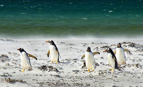
The photo (open the original) shows five gentoo penguins walking across a white sandy beach dotted with dark pebbles, with a green-blue sea behind them. Each penguin has a black back and head, a white belly and an orange beak and feet.
Mean shift on colour (with no position features) groups pixels by colour alone. Two pixels anywhere in the image join the same cluster if their colours climb to the same peak.
So a cluster is a set of colours, not a connected object. An object made of two very different colours, like a black-and-white penguin, is split between two clusters, and each of those clusters also contains every background pixel of the same colour.
Superpixels are spatially compact, and merging only joins adjacent regions. So separate black patches never merge with each other unless they touch, which is an improvement.
But the merge test is still colour similarity. A white belly touching white sand looks like one region.
A grey-level version of the scene has five kinds of pixels:
$$\text{back } 25, \quad \text{pebbles } 35, \quad \text{sea } 110, \quad \text{sand } 220, \quad \text{belly } 230 .$$Each kind is common. Run mean shift on the intensities with a flat window of radius \(h = 30\).
The windows find three peaks: near 30 (back and pebbles), at 110 (sea) and near 225 (sand and belly). Three clusters, and neither of them is "penguin".
The belly–sand edge weighs only 10, while the belly–back edge weighs 205. Any threshold that merges anything sensible merges the belly into the sand first.
Bridge to the question. The questions ask for exactly these two predictions on the real colour image. The live figure below runs both pipelines on a redrawn scene.
This method clusters pixels with similar colours together, and the number of clusters follows from the bandwidth.
The ocean would probably be segmented well, but the penguins would not. Their black regions would be clustered with the black patches of the background, and their white regions with the white regions of the background.
This method over-segments the image based on colour, then combines neighbouring regions with similar colours.
The ocean would probably be segmented well, but the penguins would not. The black regions would be segmented as separate regions, but the white regions would be merged with the background.
Both methods group by colour, and a penguin is not one colour. Neither recovers the objects. That needs knowledge of what a penguin looks like, which is what the label-based methods of lecture 20 provide.
Points worth raising in the tutorial, found while porting the notebook:
np.meshgrid(np.arange(H), np.arange(W)) has shape \((W, H)\), so after flattening the \((x, y)\) values do not belong to the pixels they are attached to (the image is \(171 \times 256\), not square). Use y, x = np.mgrid[0:H, 0:W]. It is invisible at xy_scaling = 0.005; at 1 the clusters turn into horizontal stripes (Exercise 1 figure, with false colours).xy_scaling = 0.005 the spatial term does almost nothing: the coordinates span at most about 1.3 units against a bandwidth of 25.bandwidth = 25 in cell 29.KMeans without n_init or random_state, so it prints a FutureWarning and the cluster order (and the swatch order in cell 16) changes from run to run. Cell 16 also hard-codes 4 subplots._weight_mean_color says "absolute difference", but the code takes the Euclidean norm of the RGB difference.label2rgb link points to lab2rgb.cut_normalized is not deterministic (random eigensolver start), so cell 37 can differ between runs.| Method | Key formula or rule | Parameter that matters | Output |
|---|---|---|---|
| k-means | \(J = \sum_i \lVert\mathbf x_i - \boldsymbol\mu_{c_i}\rVert^2\), assign then update | \(k\) | exactly \(k\) colour groups |
| Mean shift | \(\mathbf m(\mathbf x) = \dfrac{\sum_i \mathbf x_i g_i}{\sum_i g_i} - \mathbf x \propto \nabla \hat f_h\) | bandwidth \(h\) (and spatial \(h/s\)) | one cluster per density peak |
| SLIC | \(D = d_{lab} + \tfrac{\alpha}{S} d_{xy}\), search in \(2S \times 2S\) | \(k\), compactness \(\alpha\) | compact superpixels |
| RAG merging | merge the lowest edge while \(w < \tau\), recompute means | threshold \(\tau\) | fewer, larger regions as \(\tau\) grows |
| Normalised cut | \(\dfrac{\operatorname{cut}}{\operatorname{assoc}(A,V)} + \dfrac{\operatorname{cut}}{\operatorname{assoc}(B,V)}\) | similarity scale \(\sigma\) | balanced splits along weak edges |
| GrabCut | colour GMM likelihood \(+\ \lambda \cdot\) boundary length | box prompt, \(\lambda\) | one foreground mask |
| Mask R-CNN | detect boxes, then a binary mask per box | score threshold | instances of 80 classes |
| FCN / U-Net | per-pixel cross-entropy, skip connections, \(1\times1\) classifier | depth, input size | a class at every pixel |
| Transposed conv | multiply by \(X^{T}\); length \(s(n-1) + k\) | stride \(s\) | learned upsampling |
| SAM | focal \(+\) Dice loss, three masks per prompt | the prompt | class-agnostic masks |
| Overlap | \(\operatorname{Dice} = 2\operatorname{IoU}/(1 + \operatorname{IoU})\) | \(\operatorname{Dice} \ge \operatorname{IoU}\) |
Lecture slides: COMP90086 Computer Vision, Image Segmentation I (lecture 19) and II (lecture 20), Kris Ehinger, University of Melbourne. Notebook: worksheet11_solution-old-24.ipynb.